3 Choice under uncertainty
Forecasts are indispensable tools to make decisions under uncertainty. There are various different forecasts a method can output. In increasing order of sophistication, these are point forecasts (i.e., single number forecasts), prediction intervals and predictive distributions. Knowing when to use what is crucial, especially if we apply the forecast to ensure target service levels.
3.1 Forecasting methods
A forecast is an input to support decision-making under uncertainty. Forecasts are created by a statistical model or by human judgment. A statistical model is an algorithm, often embedded into a spreadsheet or other software, that converts data into a forecast. Of course, choosing which algorithm an organization uses for forecasting and how the organization implements this algorithm often requires the use of human judgment as well. But in the present context, we use the term “judgment” to indicate that humans influence or override a statistical forecast (see Chapter 16). Human judgment is the intuition and cognition decision-makers can employ to convert all available data and tacit information into a forecast. We discuss statistical models and human judgment in much more detail later in this book.
In reality, most forecasting processes contain elements of both judgment and statistics. A statistical forecast may serve as the basis of discussion, but this forecast is then revised in some form or other through human judgment to arrive at a consensus forecast, a combination of different existing forecasts (statistical or judgmental) within the organization. A survey of professional forecasters found that while 16% of forecasters relied exclusively on human judgment and 29% depended solely on statistical methods, the remaining 55% used either a combination of judgment and statistical forecast or a judgmentally adjusted statistical forecast (Fildes and Petropoulos, 2015). Another study of a major pharmaceutical company found that more than 50% of the forecasting experts answering the survey did not rely on the company’s statistical models when preparing their forecast (Boulaksil and Franses, 2009). Forecasting in practice is thus not an automated process. People usually influence the process. However, often the sheer number of forecasts means that not all can be inspected by humans. For instance, retail organizations may need to forecast more than 20,000 SKUs daily for hundreds or thousands of stores to drive replenishment. Naturally, forecasting at this level tends to be a more automated task, and determining which forecasts need judgmental input becomes key.
Throughout this book, we refer to a forecasting method as the process through which an organization generates a forecast. This forecast does not need to be the final consensus forecast, although some method always generates the consensus forecast. The beauty of any forecasting method is that its accuracy can be judged ex-post and compared against other methods. There is always an objective realization of demand that we can (and should) compare to the forecast to create a picture of forecast accuracy over time. Of course, we should never base this comparison on small samples. However, suppose a forecasting method repeatedly forecasts far from the actual demand realizations. In that case, this observation is evidence that the method is not working well, particularly if there is evidence that another method works better. In other words, whether a forecasting method is good or bad is not a question of belief but of scientific empirical comparison. If the forecastability of the underlying demand is challenging, then multiple methods will fail to improve accuracy. We will explore how to make such a forecasting comparison in more detail in Chapter 18.
One key distinction to keep in mind is that the forecast is not a target, a budget, a plan, or a decision. A forecast is simply an expression or belief about the likely state of the future. Targets, budgets, or plans are decisions based on forecasts, but these concepts should not be confused with the forecast itself. For example, our point forecast for demand for a particular item we want to sell on the market may be 100,000 units. However, it may make sense for us to set our sales representatives a target of selling 110,000 units to motivate them to do their best. In addition, it may also make sense to plan to order 120,000 units from our contract manufacturer since there is a chance that demand is higher. We want to balance the risk of stocking out against having excess inventory. To make the latter decision effectively, we would include data on ordering and sales costs, as well as assumptions on how customers would react to stockouts and how quickly the product may or may not become obsolete.
Single-number forecasts: point forecasts
Most firms operate with point forecasts – single numbers that express the most likely outcome on the market. Yet, we all understand that such a notion is somewhat ridiculous; the point forecast is unlikely to be realized precisely. A forecast can have immense uncertainty. Reporting only a point forecast communicates an illusion of certainty. Let us recall a famous quote by Goethe: “To be uncertain is to be uncomfortable, but to be certain is to be ridiculous.”
Prediction intervals
Point forecasts, in this sense, are misleading. It is much more valuable and complete to report forecasts in the form of a probability distribution or at least in the form of prediction intervals, that is, a “best case” and a “worst case” scenario – always with the understanding that reality may still fall outside these bounds, if only with a very small probability. The endpoints of a prediction interval are also known as quantile forecasts. For instance, a 10% quantile forecast is a number such that we expect a 10% chance that the future observation falls below it. A 90% quantile forecast is an analogous number, which will of course be higher than our 10% quantile forecast. And if we combine a 10% quantile forecast and a 90% quantile forecast, we have an 80% (\(=90\%-10\%\)) prediction interval.
Creating such prediction intervals requires a measure of uncertainty in the forecast. While we will explore this topic in detail in Chapter 4, we provide a brief and stylized introduction here. We usually express uncertainty as a standard deviation (usually abbreviated by the Greek letter \(\sigma\)). Given a history of forecast errors, measuring this uncertainty is pretty straightforward. The simplest form would be to calculate the population standard deviation (using the =STDEV.P function in Microsoft Excel) of past observed forecast errors (see Chapter 17 for a more in-depth treatment of measuring the accuracy of forecasts). Assuming that forecast errors are roughly symmetric, that is, over-forecasting is as likely and extensive as under-forecasting, we can then conceptualize the point forecast as the center (i.e., the mean, median, and most likely value, abbreviated by the Greek letter \(\mu\)) of a probability distribution, with the standard deviation \(\sigma\) measuring the spread of that probability distribution.
We illustrate these concepts in Figure 3.1. Suppose our forecasting method generated a point forecast of 500. We calculate a standard deviation of our past forecast errors as 20. We can thus conceptualize our forecast as a probability distribution with a mean of 500 and a standard deviation of 20 (in this illustration, we assumed a normal distribution, drawn with the Excel function =NORM.DIST). A probability distribution is nothing but a function that maps possible outcomes to probabilities.
For example, one could ask what the probability is that demand is between 490 and 510. The area under the distribution curve between the \(x\) values of 490 and 510 would provide the answer – or the Excel function call =NORM.DIST(510, 500, 20, TRUE)-NORM.DIST(490, 500, 20, TRUE). The result is about 38.3%: the probability of seeing demand between 490 and 510.
Given a forecasted mean and a standard deviation (and the crucial assumption of a normal distribution), we can thus calculate a 95% prediction interval, by calculating the 97.5% quantile of the distribution as the upper limit (or quantile) and the 2.5% quantile as the lower limit, which yields a theoretical coverage of \(97.5\%-2.5\%=95\%\). That is, if our assumptions are correct, we predict that 95% of future observations fall within this interval. In Excel, we can calculate these interval limits or quantile forecasts using =NORM.INV(0.025, 500, 20) and =NORM.INV(0.975, 500, 20), respectively, yielding an interval of \((460.8, 539.2)\). We can examine the effects of various changes to the input variables. For instance, increasing the standard deviation makes our assumed time series harder to forecast (compare Figure 1.1) and will make the prediction interval wider, as will increasing the target interval coverage above 95%. We immediately see how targeting a higher service level than 97.5% (the upper limit of our interval) requires a higher safety stock.
A caveat: calculated prediction intervals are often too narrow (Chatfield, 2001). One reason is that these intervals often do not include the uncertainty of choosing the correct model and the uncertainty of the environment changing. It was surprising in the recent M5 forecasting competition that prediction intervals actually had the required coverage (Makridakis, Spiliotis, Assimakopoulos, Chen, et al., 2022)!
Our prediction interval has non-integer limits. While product is sold in integer units, the upper quantile forecast is 539.2. This inconsistency is a result of using the normal distribution. This distribution is commonly used in statistics and forecasting because it makes the mathematics much simpler, and because it is usually sufficient as an approximation. Using this distribution starts causing problems if we have very slow selling items, so-called count data. See Chapter 12 for a discussion of this situation.
Note that symmetry of forecast errors is not always the case in practice. For example, items with low demand are naturally censored at zero, creating a skewed error distribution (see Chapter 12); similarly, if political influence within the organization creates an incentive to over- or under-forecast, the distribution of errors can be skewed. Chapter 17 will examine how to detect such forecast bias in more depth.
Finally, a word about terminology: prediction intervals are often confused with confidence intervals (Soyer and Hogarth, 2012). While a confidence interval represents the uncertainty about an estimate of a parameter of a distribution (i.e., the mean of the above distribution), a prediction interval represents the uncertainty about a realization from that distribution (i.e., demand taking specific values in the above distribution). The confidence interval for the mean is much smaller (depending on how many observations we used to estimate the mean) than the prediction interval characterizing the distribution. In forecasting, we almost always look at prediction intervals, not confidence intervals.
Predictive distributions
A predicted probability distribution (known either as a predictive distribution, a predictive density or a distributional forecast) thus communicates a good sense of the possible outcomes and the associated uncertainty with a forecast.
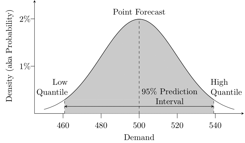
Figure 3.1: Forecasts from a probabilistic perspective
Ideally, decisions that use forecasts can work with full predictive distributions. However, how should we report such a probabilistic forecast? Usually, we do not draw the actual distribution since this may be too much information to digest for decision-makers. Reporting a standard deviation in addition to the point forecast can already be challenging to interpret. A good practice is to report 95 or 80% prediction intervals as caclulated above, that is, intervals in which we are 95 or 80% sure that demand will fall.
Prediction intervals thus provide a natural instrument for forecasters to adequately communicate the uncertainty in their forecasts and for decision-makers to decide how to manage the risk inherent in their decision. Reporting and understanding prediction intervals and predictive distributions requires some effort. However, we can automate the calculation and reporting of these intervals in modern forecasting software. Not reporting (or ignoring) the uncertainty in forecasts can have distinct disadvantages for organizational decision-making. Reading just a point forecast without a measure of uncertainty gives you no idea how much uncertainty there is in the forecast. The consequences of not making forecast uncertainty explicit can be dramatic. At best, decision-makers will judge how much uncertainty is inherent in the forecast. Since human judgment in this context generally suffers from over-confidence (Mannes and Moore, 2013), not making forecast uncertainty explicit will likely lead to under-estimating the inherent forecast uncertainty, leading to less-than-optimal safety stocks and buffers in resulting decisions. At worst, decision-makers will treat the point forecast as a deterministic number and ignore the inherent uncertainty in the forecast entirely, as well as any precautions they should take in their decisions to manage their demand risk.
Adopting prediction intervals in practice is challenging; one criticism often brought up is that it is difficult to report more than one number and that the wide range of a 95% prediction interval makes the interval almost meaningless. This line of reasoning, however, misinterprets the prediction interval. The range also contains information about probabilities since values in the center of the range are more likely than those at the end. We can easily visualize these differences, e.g., in a fan plot as in Figure 3.2, which shows a demand time series from the M5 competition (Makridakis, Spiliotis, and Assimakopoulos, 2022): areas of different shading indicate different pointwise prediction intervals. It is common to plot an inner 80% prediction band and an outer 95% prediction band as in this figure, i.e., areas in which we believe 80% respectively 95% of future observations will fall. Fan plots thus provide an easily interpreted summary of our forecast’s uncertainty and represent the state-of-the-art in communicating forecast uncertainty (Kreye et al., 2012).
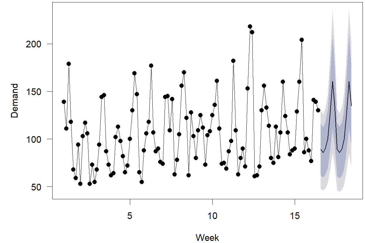
Figure 3.2: Daily demand for one SKU at one store, with point forecasts and a fan plot
Another argument against using prediction intervals is that, in the end, we need single numbers for decision-making. Ultimately, containers must be loaded with a particular volume; capacity levels require hiring a certain number of people or buying a certain number of machines. What good is a forecast showing a range when we need one number in the end? This argument makes the mistake of confusing the forecast with decision-making. The forecast is an input into a decision, not a decision per se. Firms can and must set service-level targets and solve the inherent risk trade-offs to translate probabilistic or interval forecasts into single numbers and decisions.
3.2 Forecasts and service levels
Consider the following illustrative example. Suppose you are a baker and need to decide how many bagels to bake in the morning for selling throughout the day. The variable cost to make bagels is 10 cents, and you sell them for \(\$1.50\). You donate bagels you do not sell during the day to a kitchen for the homeless. You forecast that demand for bagels for the day has a mean of 500 and a standard deviation of 80, giving you a 95% prediction interval of roughly (340, 660). How many bagels should you bake in the morning? Your point forecast is 500 – but you probably realize this would not be the correct number. Baking 500 bagels would give you just a 50% chance of meeting all demand during the day.
This 50% chance represents an essential concept in this decision context – the so-called type I service level or in-stock probability, that is, the likelihood of meeting all demands with your inventory (see textbooks on inventory control, such as Silver et al., 2017, on different notions of service levels). This chance of not encountering a stockout is a crucial metric often used in organizational decision-making. What service level should you strive to obtain? The answer to that question requires carefully comparing the implications of running out of stock with the repercussions of having leftover inventory – that is, managing the inherent demand risk. The key factors here are so-called overage and underage cost, that is, assessing what happens when too much or too little inventory is available.
An overage situation in the case of our bagel baker implies that they have made bagels at the cost of 10 cents that they are giving away for free; this would lead to a loss of 10 cents. An underage situation implies that they have not made enough bagels and thus lose a profit margin of \(\$1.40\) per bagel not sold. This underage cost is an opportunity cost – a loss of \(\$1.40\). Assuming no other expenses of a stockout (i.e., loss of cross-sales, loss of goodwill, loss of reputation, etc.), this \(\$1.40\) represents the total underage cost in this situation. Underage costs, in this case (\(\$1.40\)), are much higher than overage costs (10 cents), implying that you would probably bake more than 500 bagels in the morning.
Finding the right service level in this context is known as the newsvendor problem in the academic literature (Qin et al., 2011). Its solution is simple and elegant. One calculates the so-called critical fractile, the ratio of underage to the sum of underage and overage costs. In our case, this critical fractile roughly equals \(93\%\) (=1.40/[1.40+0.10]). The critical fractile is the optimal type I service level. In other words, considering the underage and overage costs, you should strive for a 93% service level in bagel baking. In the long run, this service level balances the opportunity costs of running out of stock with the obsolescence costs of baking bagels that do not sell.
So how many bagels should you bake? We have seen above how to calculate this in Microsoft Excel: the formula =NORM.INV(0.93, 500, 80) gives us a result of about 618. In other words, you should bake 618 bagels to have a 93% chance of meeting all demand in a day, which is the optimal target service level.
This example illustrates the difference between the forecast, which serves as an input into a decision, and the actual decision, which is the number of bagels to bake. The point forecast is not the decision, and making a good decision would be impossible without understanding the uncertainty inherent in the point forecast. Good decision-making under uncertainty requires understanding uncertainty and balancing risks. In addition, while forecasts are crucial ingredients for decision-making, there are always additional inputs, usually in the form of costs and revenues. In the case of our bagel baker, the critical managerial task was not to influence the forecast but to understand the cost factors involved with different risks in the decision and then define a service level that balances these risk factors. A good forecast in the form of a probability distribution or a prediction interval should make this task easier. The actual quantity of bagels baked is simply a function of the forecast and the target service level derived from the cost structure.
Our discussion highlights the importance of setting adequate service levels for the items in question. Decision-makers should understand how their organization derives these service levels. Since the optimal service level depends on the product’s profit margin, items with different profit margins require different service levels. While overage costs are comparatively easy to measure (cost of warehousing, depreciation, insurance, etc.; see Timme and Williams-Timme, 2003), underage costs involve understanding customer behavior and are thus more challenging to quantify. What happens when a customer desires a product that is not available? In the best case, the customer finds and buys a substitute product, which may even be sold at a higher margin, or puts the item on backorder. In the worst case, customers take their business elsewhere and tweet about the bad service experience. Studies of a mail-order-catalog business show that the indirect costs of a stockout – the opportunity costs from lost cross-sales and reduced long-term sales of the customer – are almost twice as high as the lost revenue from the stockout itself (Anderson et al., 2006). Similar consequences of stockouts threaten the profitability of supermarkets (Corsten and Gruen, 2004). Setting service levels thus requires studying customer behavior and understanding the revenue risks associated with a stockout. Since this challenge can appear daunting, managers can sometimes react in a knee-jerk fashion and set very high service levels, e.g., 99.99%. Such an approach leads to excessive inventory levels and related inventory-holding costs. Achieving the right balance between customer service and inventory holding requires a careful analysis and thorough understanding of the business.
Note that while we use inventory management as an example of decision-making under uncertainty, a similar rationale for differentiating between forecast and related decision-making also applies in other contexts. For example, in service staffing decisions, the forecast relates to customer demand in a specific time period. The decision is how much service capacity to put in place. Too much capacity means resources wasted in firms. Too little capacity means wait times and possibly lost sales due to customers avoiding the service system due to inconvenient queues. Similarly, in project management, a forecast may involve predicting how long the project will take and finding how much time buffer we need to build into the schedule. Too large a buffer may result in wasted resources and lost revenue, whereas too little buffer may lead to projects exceeding their deadlines and resulting in contractual fines. One must understand that forecasting by itself is not risk management – forecasting simply supports managers in making decisions by carefully balancing the risk inherent in their choice under uncertainty.
Existing inventory management systems are more complex than examples in this chapter may suggest, since they require adjusting for fixed costs of ordering (i.e., shipping and container filling), uncertain supply lead times (e.g., by ordering from overseas), best-by dates and obsolescence, optimization possibilities (like rebates or discounts on large orders), contractually agreed order quantities, as well as dependent demand items (i.e., scheduling production for one unit requires ordering the whole bill of materials). A thorough review of inventory management techniques is beyond the scope of this book, and we refer interested readers to Nahmias and Olsen (2015), Silver et al. (2017) or Syntetos et al. (2016) for comprehensive information.
Key takeaways
Forecasts are not targets, budgets, plans, or decisions; these are different concepts that need to be kept apart within organizations, or confusion will occur.
Often the word forecast is shorthand for point forecast. However, point forecasts are seldom perfectly accurate. We need to measure and communicate the uncertainty associated with our forecast. To accomplish this, we calculate prediction intervals or predictive densities, which we can visualize using fan plots.
A key concept to convert a forecast into a decision is the service level, that is, the likelihood of meeting an uncertain demand with a fixed quantity. Target service levels represent critical managerial decisions and should balance the risk of not having enough units available (underage) and having too many units (overage).