9 Exponential smoothing
One of the most accurate and robust methods for time series forecasting is Exponential Smoothing. Its performance advantage was established in the M3 forecasting competition, which compared more than 20 forecasting methods for their performance across 3,003 time series from different industries and contexts (Makridakis and Hibon, 2000). You might think that in the 20 years since the M3 competition, more modern methods, like the ones based on Artificial Intelligence and Machine Learning (see Chapter 14), would have caught up to this venerable method. Surprisingly, this is not the case. Exponential Smoothing was still competitive in the more recent M5 competition, outperforming 92.5% of all submissions (Kolassa, 2022a; Makridakis, Spiliotis, and Assimakopoulos, 2022). In a world of rapid innovation and research, a method that has been around at least since the 1950s still shines.
9.1 Change and noise
There is extensive theoretical work on Exponential Smoothing. The method is optimal (i.e., it will minimize expected squared forecast errors) for random walks with noise and various other time series models (Chatfield et al., 2001; Gardner, 2006). Further, what was once a rather ad-hoc methodology is now formalized in a state space framework (Hyndman et al., 2008). Exponential Smoothing is not only an accurate, versatile, and robust method. It is also intuitive and easy to understand and interpret. Another important aspect of the method is that the data storage and computational requirements for Exponential Smoothing are minimal. We can easily apply this method to many time series in real time.
To illustrate how Exponential Smoothing works, we begin with a simple time series without trend and seasonality. In such a series, variance in demand from period to period is driven either by random changes to the level (i.e., long-term shocks to the time series) or by random noise (i.e., short-term shocks to the time series). The essential forecasting task then becomes estimating the level of the series in each period and using that level as a forecast for the next period. The key to effectively estimating the level in each period is to differentiate level changes from random noise (i.e., long-term shocks from short-term shocks).
As discussed in Section 7.3, if we believe that there are no random-level changes in the time series (i.e., the series is stable), then our best estimate of the level involves using all of our available data by calculating a long-run average over the whole time series. If we believe there is no random noise in the series (i.e., we can observe the level), then our estimate of the level is simply the most recent observation, discounting everything that happens further in the past. Not surprisingly, the right thing to do in a time series containing both random-level changes and random noise is something in between these two extremes: calculate a weighted average over all available data, with weights decreasing the further we go back in time. This approach to forecasting, in essence, is Exponential Smoothing.
Let the index \(t\) describe the period of a time series. We update the level estimate (\(= \mathit{Level}\)) in each period \(t\) according to Exponential Smoothing as follows:
\[\begin{align} \mathit{Level}_{t} = \mathit{Level}_{t-1} + \alpha \times \mathit{Forecast~Error}_{t}. \tag{9.1} \end{align}\]
In this equation, the coefficient \(\alpha\) (alpha) is a smoothing parameter and lies somewhere between 0 and 1 (we will pick up the topic of what value to choose for \(\alpha\) later in this chapter). The Forecast Error in period \(t\) is simply the difference between the actual demand (= Demand) in period \(t\) and the forecast made for the period \(t\):
\[\begin{align} \mathit{Forecast~Error}_{t} = \mathit{Demand}_{t} - \mathit{Forecast}_{t}. \tag{9.2} \end{align}\]
In other words, Exponential Smoothing follows the simple logic of feedback and response. The forecaster estimates the current time series level, which they use as the forecast. This forecast is then compared to the actual demand in the series in the next period. This assessment allows the forecaster to revise the level estimate according to the discrepancy between the forecast and actual demand. The forecast for the next period is then simply the current level estimate since we assumed a time series without trend and seasonality, that is:
\[\begin{align} \mathit{Forecast}_{t+1} = \mathit{Level}_{t}. \tag{9.3} \end{align}\]
Substituting Equations (9.2) and (9.3) into Equation (9.1), we obtain
\[\begin{align} \mathit{Level}_{t} & = \mathit{Forecast}_{t} + \alpha \times \left(\mathit{Demand}_{t} - \mathit{Forecast}_{t}\right) \\ & = \left(1-\alpha\right) \times \mathit{Forecast}_{t} + \alpha \times \mathit{Demand}_{t}. \tag{9.4} \end{align}\]
We can, therefore, also interpret Exponential Smoothing as a weighted average between our previous forecasts and the currently observed demand.
Curious readers have probably noticed that the method suffers from a chicken-or-egg problem: Creating an Exponential Smoothing forecast requires a previous forecast, which naturally creates the question of how to initialize the level component. Different initializations are possible, ranging from the first observed demand data point, an average of the first few demand points, to the overall average demand.
We can convert Equation (9.4) into a weighted average over all past demand observations, where the weight of a demand observation that is \(i\) periods away from the present is as follows:
\[\begin{align} \mathit{Weight}_{i} = \alpha \times \left(1 - \alpha \right)^{i} \tag{9.5} \end{align}\]
Equation (9.5) implies an exponential decay in the weight attached to a particular demand observation the further this observation lies in the past. The technique is called Exponential Smoothing because of exponential decay. Figure 9.1 shows the weights assigned to past demand observations for typical values of \(\alpha\). We see that higher values of \(\alpha\) yield weight curves that drop faster as we go into the past. The more recent history receives more weight than the more distant past if \(\alpha\) is higher. Thus, forecasts will be more adaptive to changes for higher values of \(\alpha\). Note that the weight assigned under Exponential Smoothing to a period in the distant past can become very small (particularly with a high \(\alpha\)) but remains positive nonetheless. We further discuss how to set the value of \(\alpha\) in Section 9.2 below.
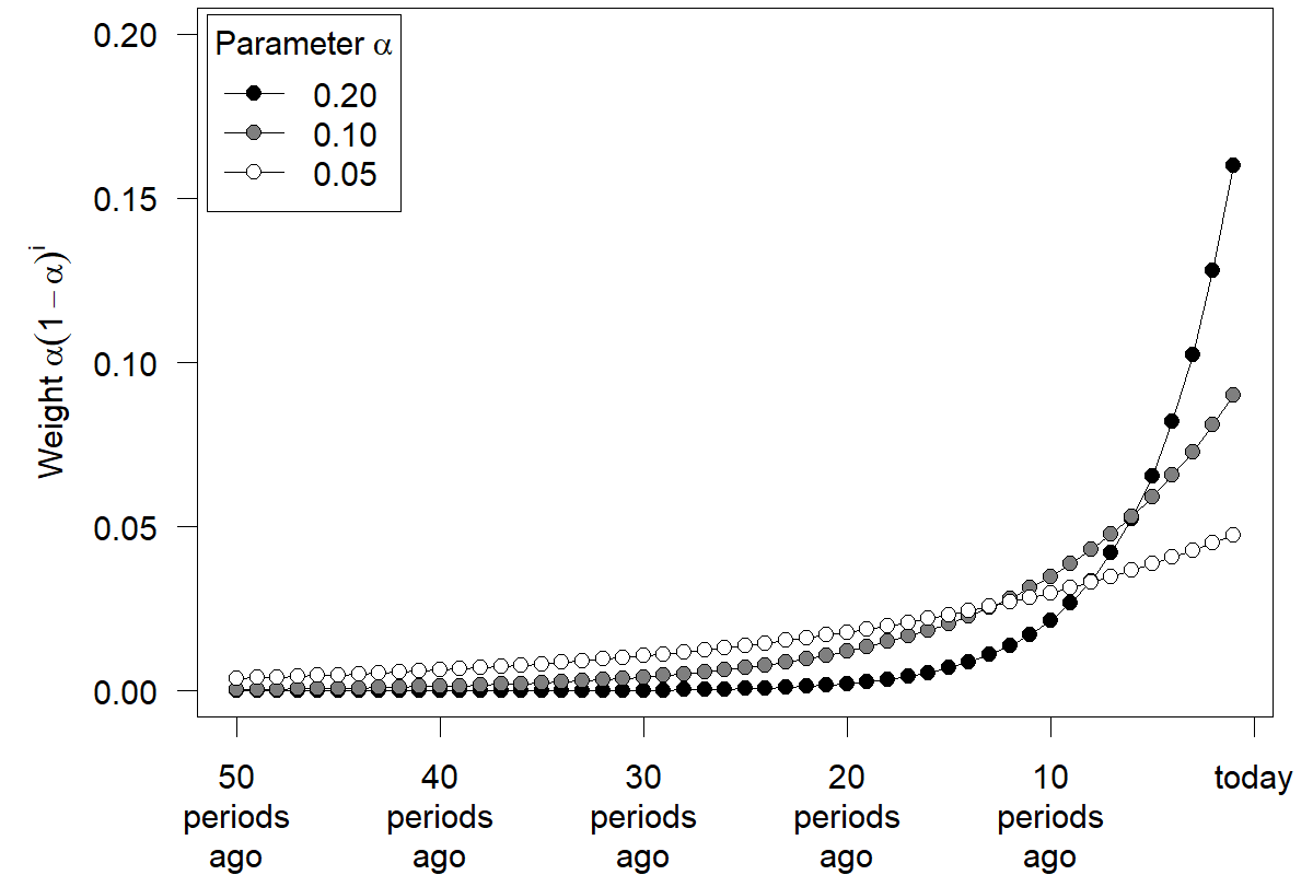
Figure 9.1: Weights for past demand under Exponential Smoothing
Forecasts created through Exponential Smoothing can thus be considered a weighted average of all past demand data. The weight associated with each demand decays exponentially the more distant a demand observation is from the present. It is essential, though, that one does not have to calculate a weighted average over all past demand to apply Exponential Smoothing. As long as a forecaster consistently follows Equation (9.1), all that is needed is a memory of the most recent forecast and an observation of actual demand to update the level estimate. Therefore, the data storage and retrieval requirements for Exponential Smoothing are extremely low. Consistently applying the method generates forecasts as if one were calculating a weighted average over all past demand with exponentially decaying weights in each period, as shown in Figure 9.1.
Forecasters sometimes use moving averages as an alternative to Exponential Smoothing. In a moving average of size n, the most recent n demand observations are averaged with equal weights to create a forecast for the future. This method is essentially similar to calculating a weighted average over all past demand observations, with the most recent n observations receiving equal weights and all others receiving zero weight.
However, why should there be such a step change in weighing past demands? Under Exponential Smoothing, all past demand observations receive some weight. This weight decays the more you move into the past. But moving averages assign equal weights for a while and no weight to the more extended demand history. An observation, e.g., six periods ago, might receive the same weight as the most recent observation, but an observation seven periods ago receives no weight. This radical change in weights from one period to the next makes moving averages appear arbitrary.
9.2 Optimal smoothing parameters
The choice of the right smoothing parameter \(\alpha\) in Exponential Smoothing is undoubtedly essential. Conceptually, a high \(\alpha\) corresponds to a belief that variation in the time series is primarily due to random changes in the level; a low \(\alpha\) corresponds to a belief that this variation in the series is mainly due to random noise. If \(\alpha=1\), Equation (9.4) shows that the new level estimated after observing a demand is precisely equal to that last observed demand. That is, for \(\alpha=1\), the next forecast will be the previously observed demand, i.e., we have a naive forecast (compare Section 8.2), which would be appropriate for series 2 in Figure 7.3. As \(\alpha\) becomes smaller, the new level estimate will become more and more similar to a long-run average. A long-run average would be correct for a stable time series such as series 1 in Figure 7.3. In the extreme, if \(\alpha=0\), per Equation (9.1) we will never update our estimate of the level, so the forecast will be completely non-adaptive and only depend on how we originally initialized this Level variable.
Choosing the right \(\alpha\) thus corresponds to selecting the type of time series that our focal time series resembles more; series that look more like series 1 in Figure 7.3 should receive a higher \(\alpha\); series that look more like series 2 should receive a lower \(\alpha\). In practice, forecasters do not need to make this choice. They can rely on optimization procedures that will fit Exponential Smoothing models to past data, minimizing the discrepancy between hypothetical past forecasts and actual past demand observations by changing the \(\alpha\). The output of this optimization is a good smoothing parameter to use for forecasting. We can interpret the smoothing parameter as a measure of how much the demand environment in the past has changed over time. High values of \(\alpha\) mean the market was very volatile and constantly changing, whereas low values of \(\alpha\) imply a relatively stable market with little persistent change. In demand forecasting, smaller values of \(\alpha\), up to about \(\alpha=0.2\), typically work well since demand usually does have an underlying level that is relatively stable. In contrast, stock prices typically exhibit more random-walk-like behavior, corresponding to higher \(\alpha\).
9.3 Extensions
The simple incarnation of Exponential Smoothing described in Section 9.1 is often called Single Exponential Smoothing (SES), or Simple Exponential Smoothing because it is the simplest version of Exponential Smoothing one can use, and because it has a single component, the level, and a single smoothing parameter \(\alpha\). One can extend the logic of Exponential Smoothing to forecast more complex time series. Take, for example, a time series with an (additive) trend and no seasonality. In this case, one proceeds with updating the level estimate per Equation (9.1), but then additionally estimates the trend in period \(t\) as follows:
\[\begin{align} \mathit{Trend}_{t} & = \left(1 - \beta\right) \times \mathit{Trend}_{t-1}+ \beta \times \left(\mathit{Level}_{t} - \mathit{Level}_{t-1}\right) \tag{9.6} \end{align}\]
This method is also referred to as Holt’s method. Notice the similarity between Equations (9.4) and (9.6). In Equation (9.6), beta (\(\beta\)) is another smoothing parameter that captures the degree to which a forecaster believes that the trend of a time series is changing. A high \(\beta\) would indicate a trend that can rapidly change over time, and a low \(\beta\) would correspond to a more or less stable trend. We again need to initialize the trend component to start the forecasting method, for example, by taking the difference between the first two demands or calculating the average trend over the entire demand history. Given that we assumed an additive trend, the resulting one-period-ahead forecast is then provided by
\[\begin{align} \mathit{Forecast}_{t+1} = \mathit{Level}_{t} + \mathit{Trend}_{t} \tag{9.7} \end{align}\]
Usually, forecasters need not only to predict one period ahead into the future, but longer forecasting horizons are necessary for successful planning. In production planning, for example, the required forecast horizon is given by the maximum lead time among all suppliers for a product – often as far out as 6 to 8 months. Exponential Smoothing easily extends to forecasts further into the future as well; for example, in this case of a model with additive trend and no seasonality, the \(h\)-step-ahead forecast into the future is calculated as follows:
\[\begin{align} \mathit{Forecast}_{t+h} = \mathit{Level}_{t} + h \times \mathit{Trend}_{t} \tag{9.8} \end{align}\]
This discussion requires emphasizing a critical insight and common mistake for those not versed in applying forecasting methods: Estimates are only updated if new information is available. We cannot meaningfully update level or trend estimates after making the one-step-ahead forecast and before making the two-step-ahead forecast. Thus, we use the same level and trend estimates to project the one-step-ahead and the two-step-ahead forecasts at period \(t\). In the extreme, in smoothing models without a trend or seasonality, this means that all forecasts for future periods are the same; that is, if we expect the time series to be a level only time series without a trend or seasonality, we estimate the level once. That estimate becomes our best guess for demand in all future periods.
Of course, we understand that this forecast will get less accurate the more we project into the future, owing to the potential instability of the time series (a topic we have explored already in Chapter 4). Still, this expectation does not change the fact that we cannot derive a better estimate of what happens further in the future at the current time. After observing the following period, new data becomes available, and we can again update our estimates of the level and, thus, our forecasts for the future. Therefore, the two-step-ahead forecast made in period \(t\) (for period \(t+2\)) usually differs from the one-step-ahead forecast made in period \(t+1\) (for the same period \(t+2\)).
A trended Exponential Smoothing forecast extrapolates trends indefinitely. This aspect of the model could be unrealistic for long-range forecasts. For instance, if we detect a negative (downward) trend, extrapolating this trend out will eventually yield negative demand forecasts. Or assume that we are forecasting market penetration and find an upward trend – in this case, if we forecast out far enough, we will get forecasts of market penetration above 100%. Thus, we always need to truncate trended forecasts appropriately. In addition, few processes grow without bounds, and it is often better to dampen the trend component as we project it into the future. Such trend dampening will not make a big difference for short-range forecasting but will strongly influence, and typically improve, long-range forecasting (Gardner and Mckenzie, 1985).
Similar extensions allow Exponential Smoothing to apply to time series with seasonality. Seasonality parameters are estimated separately from the trend and level components. We use an additional smoothing parameter \(\gamma\) (gamma) to reflect the degree of confidence a forecaster has that the seasonality in the time series remains stable over time. With additive trend and seasonality, we refer to such an Exponential Smoothing approach as Holt–Winters Exponential Smoothing.
Outliers can unduly influence the optimization of smoothing parameters in Exponential Smoothing models. Fortunately, these data problems are now well understood, and reasonable solutions allow forecasters to automatically pre-filter and replace unusual observations in the dataset before estimating smoothing model parameters (Gelper et al., 2009).
In summary, we can generalize Exponential Smoothing to many different forms of time series. A priori, it is sometimes unclear which Exponential Smoothing model to use; however, one can run a forecasting competition to determine which model works best on past data (see Chapter 18). In this context, the innovation state space framework for Exponential Smoothing is usually applied (Hyndman et al., 2008). This framework differentiates between five different variants of trends in time series (none, additive, additive dampened, multiplicative, multiplicative dampened) and three different variants of seasonality (none, additive, multiplicative). Further, we can conceptualize random errors as either additive or multiplicative. As a result, \(5\times3\times2 = 30\) different versions of Exponential Smoothing are possible; this catalog of models is sometimes referred to as Pegels’ classification. Models are referred to by three letters, the error (A or M), the trend (N, A, Ad, M, or Md, where Ad and Md stand for dampened versions), and the seasonality (N, A, or M), and each version’s formulas for applying the Exponential Smoothing logic are well known (Gardner, 2006; Hyndman and Athanasopoulos, 2021). To make this framework work, one can define a hold-out sample, i.e., a sub-portion of the data available, and fit each of these 30 models to the data in the hold-out sample. One can then test the performance of each fitted model in the remaining data and select the one that works best. Alternatively, one can use information criteria in-sample to choose the best fitting model.
Using all 30 models in Pegel’s classification may be excessive, and some models may be unstable, especially those combining multiple multiplicative components. A reduced set, including eight Exponential Smoothing models (ANN, ANA, AAdN, AAdA, MNN, MNM, MadN, and MAdM), is efficient and effective in large-scale tests (Fotios Petropoulos et al., 2023). For example, when compared against the complete set of 30 models in more than 50,000 time series from the M competition data, using just these eight models decreases the MASE (see Section 17.2) from 1.046 to 0.942 and cuts the computational time to about 1/3. In other words, these eight models seem to fit most forecasting situations well.
Exponential Smoothing is implemented in the forecast (Hyndman et al., 2023), the smooth (Svetunkov, 2023), and the fable (O’Hara-Wild et al., 2020) packages for R, under the name of “ETS”, which stands for error, trend and seasonality. [More precisely, what is implemented is the more abstract state space formulation discussed above.] This is a very sophisticated implementation that will automatically choose the (hopefully) best model out of the full classification of Gardner (2006), and that will automatically optimize the smoothing parameters. There are also various specific Exponential Smoothing models implemented across multiple other R packages, but we would always recommend going with forecast and fable.
In Python, Exponential Smoothing is implemented in various classes in the statsmodels package (Perktold et al., 2022). There is no unified framework as with ETS in the R packages, so you will need to assess each model on its merits yourself; however, the statsmodels classes do optimize the smoothing parameters.
Key takeaways
Exponential Smoothing is a simple and surprisingly effective forecasting technique. It can model trend and seasonality components.
Exponential Smoothing can be interpreted as feedback-response learning, as a weighted average between the most recent forecast and demand, or as a weighted average of all past demand observations with exponentially declining weights. All three interpretations are equivalent.
Your software will usually determine the optimal Exponential Smoothing model as well as the smoothing parameters automatically. High parameters imply that components change quickly over time; low parameters imply relatively stable components.
Trends will be extrapolated indefinitely. Consider dampening trends for long-range forecasts. Do not include trends in your model unless you have solid evidence that a trend exists.
There are up to 30 different forms of Exponential Smoothing models, although only a smaller subset of them are broadly relevant; modern software will usually select which of these works best in a time series using an estimation sample or information criteria.