7 Time series decomposition
A very simple but often surprisingly effective way to forecast is to decompose a series into the components we encountered in the previous chapter, forecast each component separately, and combine the forecasts back together.
7.1 The purpose of decomposition
Decomposition is a management technique for complexity reduction. Separating a problem into its components and solving them independently before reassembling them into a broader decision enables better decision-making (e.g., Raiffa, 1968).
The decomposition of univariate time series data is a standard tool many organizations use. It creates a cleaner picture of our time series, allowing us to better spot the tree within a forest. Here is why this can be helpful:
Decomposition provides a clean way to identify the trend and seasonality components. We may suspect that the trend requires dampening or that seasonality changes over time. Decomposition helps to check your assumptions.
Decomposition allows us to identify your series’ causal drivers. For example, holidays or a football match can impact demand. Seasonality can obfuscate the effect of such events in our data. Removing seasonality through decomposition will thus allow us to identify the impact of such special events more easily.
Decomposition may alert us that two different types of seasonality influence your data (see Chapter 15). For example, when looking at daily data, the effects of the weekday may become more salient once we remove the monthly impact.
Decomposition enables us to spot outliers. Time series may contain outliers (i.e., anomalies) that are difficult to spot. Since decomposition removes systematic variation, outliers become easier to detect in the remainder.
Decomposition allows us to create a seasonally adjusted series. For instance, governments want to understand and communicate the unemployment rate over time. Unemployment can be very seasonal, for example, due to a winter construction work slowdown. If we do not seasonally adjust a reported time series, readers might misinterpret an increase in the unemployment rate as substantive rather than driven by the season.
Decomposition can be used in forecasting. The technique provides a structured way of thinking about a time series forecasting problem. The key idea is to decompose a time series into separate components that can be examined, estimated, and forecasted separately. We can then recombine the component forecasts into a regular forecast. Many forecasting methods require data that has already been decomposed or incorporate a decomposition approach directly into the method.
7.2 Decomposition methods
We can use a decomposition method to decompose the time series data into trend, seasonality, and remainder. To reconstruct the data, these components can be added or multiplied. In the former case, we get \(\text{data} = \text{trend} + \text{seasonal} + \text{remainder}\), and in the latter, \(\text{data} = \text{trend} \times \text{seasonal} \times \text{remainder}\). Figure 7.1 illustrates an original time series at the top that is decomposed into trend, seasonal, and remainder components using an additive method.
The remainder is whatever remains in the time series after removing trend and seasonality. If trend and seasonality capture all systematic variation in the data, then the remainder will only contain random noise. Otherwise, it will also include some systematic information, so any pattern visible in the remainder series can be very informative.
Historically, people tried to model the business cycle as an additional component. But since estimating the business cycle and predicting when the cycle turns is inherently very challenging, many methods nowadays do not explicitly consider the business cycle as a separate component. In addition, the trend component often captures the business cycle sufficiently well.
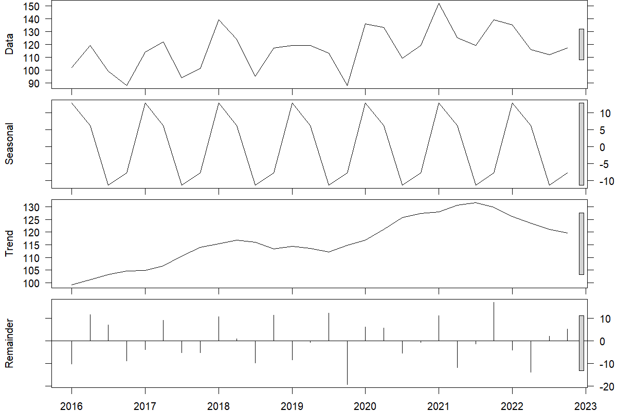
Figure 7.1: An original quarterly time series (top) along with the estimated seasonality, trend, and remainder
When interpreting publicly available time series, such as data from the Bureau of Labor Statistics, one needs to carefully understand whether or not seasonality has already been removed from the data. Most government data is reported as seasonally adjusted, implying that the seasonal component has been removed from the series. This decomposition is usually applied to the time series to avoid readers over-interpreting month-to-month seasonal changes.
Most commercial software offers methods to remove seasonality and trends from a time series. Taking seasonality and trends out of a time series is also easy in spreadsheet modeling software such as Microsoft Excel. Take monthly data as an example. As a first step, calculate the average demand over all data points and then calculate the average demand for each month (i.e., average demand in January, February, etc.). Dividing the average monthly demand by the overall average demand creates a seasonal index. Then dividing all demand observations in the time series by the corresponding seasonal index creates a deseasonalized series. We illustrate the results of such a seasonal adjustment in Figure 7.2.
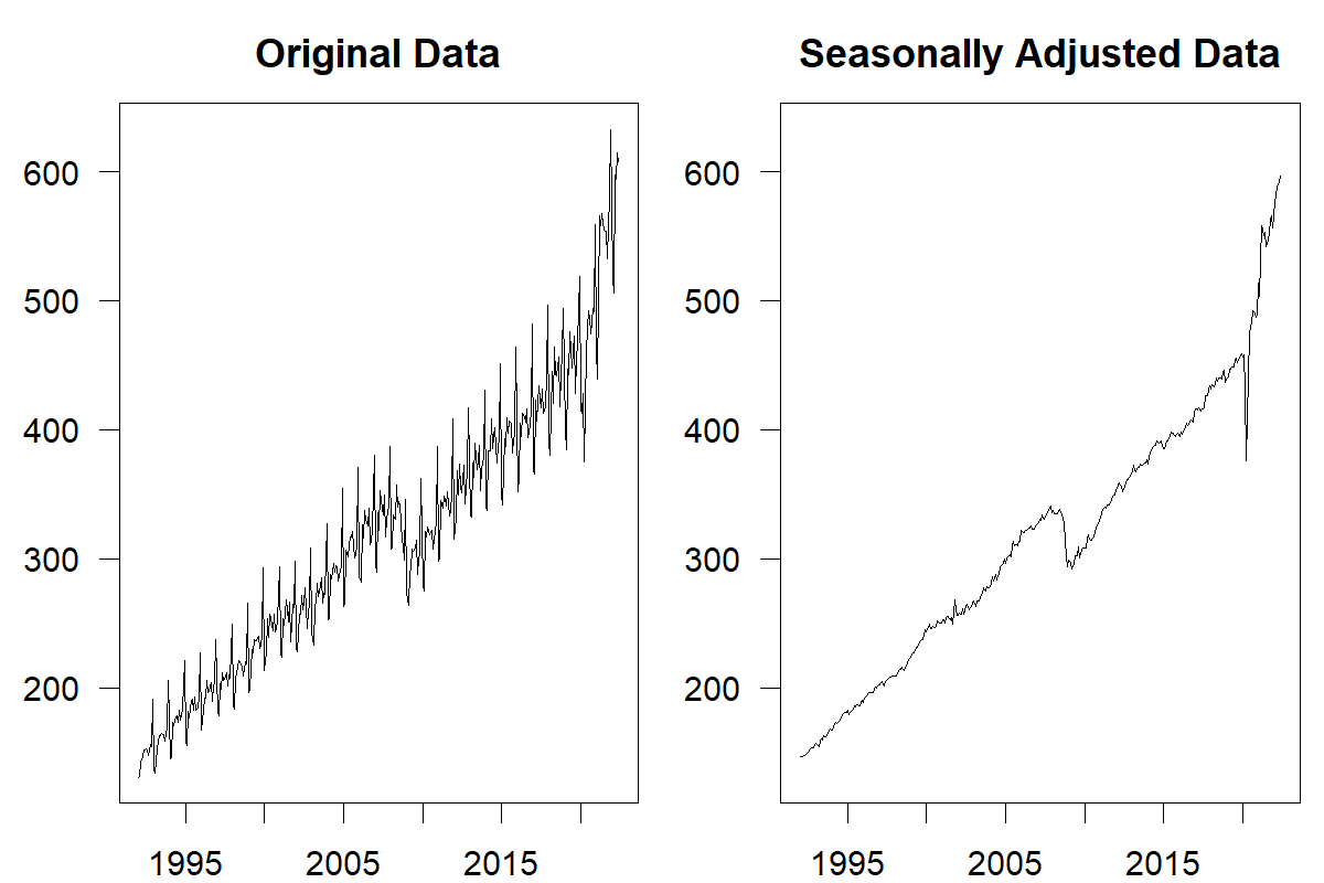
Figure 7.2: Monthly US retail sales 1992–2022 (Source: US Census Bureau, https://www.census.gov/retail/index.html)
Similarly, data can be detrended by first calculating the average difference between successive observations of the series and then subtracting \((n-1)\) times this average from the \(n\)th observation in the time series. For example, take the following time series: 100, 120, 140, and 160. The first differences of the series are 20, 20, and 20, with an average of 20. The detrended series is thus \(100 - 0 \times 20 = 100\), \(120 - 1 \times 20 = 100\), \(140 - 2 \times 20 - 100\), and \(160 - 3 \times 20 = 100\).
While these methods of deseasonalizing and detrending data are simple to use and understand, they suffer several drawbacks. For instance, they do not allow seasonality indices and trends to change, making their application challenging for more extended time series. Figure 7.2 illustrates an example of this problem. While initially, our method of deseasonalizing the data removed seasonality from the series, the later part of the series exhibits a seasonal pattern again since the seasonal indices have changed. In shorter time series, outlier data can also strongly influence decomposition methods. More sophisticated (and complex) methods have been developed for these reasons. The Bureau of Labor Statistics has developed an algorithm called X-13ARIMA-SEATS (US Census Bureau, n.d.). Software implementing this algorithm is available to download for free from the Bureau’s website.
Most time series decomposition methods are designed for monthly and quarterly data, with few tools available for daily and sub-daily series. For instance, hospitals record hourly patient arrivals in their services, typically showing a time-of-day pattern, a day-of-week pattern, and a time-of-year pattern (see Chapter 15). These seasonalities may also interact with special events such as holidays and sports events. One time series decomposition method for such high-frequency time series (e.g., hourly and daily) is the STL (seasonal-trend decomposition based on loess) procedure (Cleveland et al., 1990). An extension of the STL procedure, Multiple Seasonal-Trend decomposition using Loess (MSTL) can be used to decompose time series with multiple seasonal patterns (Bandara et al., 2021).
7.3 Stability of components
The observation that seasonal components can change leads to a critical discussion. The real challenge of time series analysis lies in understanding the stability of the components of a series. A perfectly stable time series is a series where the components do not change as time progresses – the level only increases through the trend, and the trend remains constant. The seasonality remains the same from year to year. If true, the best time series forecasting method works with long-run averages. Yet time series often are inherently unstable, and components change over time. The level of a series can abruptly shift as new competitors enter the market. The trend of a series can evolve as the product moves through its lifecycle. Even the seasonality of a series can change if underlying consumption or promotion patterns shift throughout the year.
To illustrate what change means for a time series and the implications that change has for time series forecasting, consider the two illustrative and artificially constructed time series in Figure 7.3. Both are time series without trends and seasonality (or deseasonalized and detrended already). Series 1 is a perfectly stable series, such that month-to-month variation resembles only random noise. This example comes from a stationary demand distribution and is typical for mature products. Series 2 is a time series that is highly unstable, such that month-to-month variation resembles only change in the underlying level. This example of data stems from a so-called random walk and is typical for prices in an efficient market. We used the same random draws to construct both series; in series 1, randomness represents just random noise around a stable level (around 500 units). The best forecast for this series would be a long-run average (i.e., 500). In series 2, randomness represents random changes in the unstable level, which can push the level of the time series up or down by the nature of randomness. The best forecast in this series would be the most recent demand observation. The same randomness can create two very different types of time series requiring very different approaches to forecasting.
In other words, uncertain but stable time series can use all available data to estimate the time series component and create a forecast. In unstable time series, we place a lot of weight on very recent data, and very distal data has very little weight in generating forecasts. Differentiating between stable and unstable components, and thus using or discounting past data, is the fundamental principle underlying Exponential Smoothing, which is a technique we will introduce in Chapter 9, while the “extreme” cases of purely stable or unstable series motivate the consideration of simple forecasting methods (see Chapter 8).
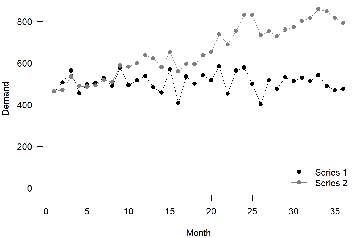
Figure 7.3: A stable and an unstable time series
Key takeaways
In time series decomposition, we separate a series into its seasonal, trend, level, and remainder components. We analyze these components separately and finally combine the pieces to create a forecast.
Components can be decomposed and recombined additively or multiplicatively.
Multiplicative components increase growth/decline patterns over time, whereas additive components imply a more linear growth/decline.
The challenge of time series modeling lies in understanding how much the time series components change over time.