17 Error measures
So far, we have studied several forecasting algorithms. Most of these can have many variants, depending on whether we include seasonality, trend, or other components. How do we establish whether one algorithm does a better job at forecasting a given time series than another one? We need to benchmark different forecasting methods and find the best-performing ones. We thus need forecast quality key performance indices or error measures. This chapter examines the most common error measures for point forecasts and also briefly introduces such KPIs for prediction intervals and predictive densities.
Performance measurement is necessary for management; it is hard to set goals and coordinate activities if we do not measure performance. This statement is true for almost any aspect of a business, but particularly so for forecasting. However, it contradicts how society often treats forecasting (Tetlock and Gardner, 2015). Pundits on television can make bold statements about the future without their feet being held to the fire; management gurus are praised when one of their predictions has come true, without ever considering their long-run record. A similar culture can exist in organizations – managerial gut judgments are taken as fact without ever establishing whether the forecaster making the judgment has a history of being spot on or mostly off. Even worse, forecasts are often made in ways that it becomes impossible to examine their quality, particularly if the forecast does not include a proper time frame.
The good news is that in demand forecasting, forecasts are usually quantified (“we expect demand for SKU X to be Y”) and come within a time frame (“Z months from now”). Such a specificity allows explicitly calculating the error in the forecast and thus making long-run assessments of this error. Nevertheless, deciding whether a demand forecast is “good” or one forecasting algorithm is “better” than another is not entirely straightforward. We will devote this chapter to the topic.
17.1 Bias and accuracy
This section introduces the concepts of bias and accuracy in forecast error measurement and provides an overview of commonly used metrics. Suppose we have calculated a single point forecast and observe the corresponding demand realization later. We will define the corresponding error as
\[\begin{align} \mathit{Error} = \mathit{Forecast}-\mathit{Demand}. \tag{17.1} \end{align}\]
For instance, if \(\mathit{Forecast} = 10\) and \(\mathit{Demand} = 8\), then \(\mathit{Error} = 10 - 8 = 2\). This definition has the advantage that over-forecasts (i.e., \(\mathit{Forecast}>\mathit{Demand}\)) correspond to positive errors, while under-forecasts (i.e., \(\mathit{Forecast} < \mathit{Demand}\)) correspond to negative errors, which follows everyday intuition.
With a slight rearrangement, this definition means that
\[\begin{align} \mathit{Demand} = \mathit{Forecast}-\mathit{Error}. \tag{17.2} \end{align}\]
or “actuals equal the model minus the error,” instead of “plus.” The “plus” convention is common in statistics and machine learning, where one would define the error as \(\mathit{Error} = \mathit{Demand} - \mathit{Forecast}\). Such a definition yields the unintuitive fact that over-forecasts (or under-forecasts) would correspond to negative (or positive) errors.
Our error definition, although common, is not universally accepted in forecasting research and practice, and many forecasters adopt the alternative error definition motivated by statistics and machine learning. Green and Tashman (2008) surveyed practicing forecasters about their favorite error definition. Even our definition of forecast error in Chapter 9 defines the error in its alternate form – mostly because this alternative definition makes Exponential Smoothing easier to explain and understand.
Whichever convention you adopt in your practical forecasting work, the key takeaway is that whenever you discuss errors, you must ensure everyone is using the same definition. Note that this challenge does not arise if we are only interested in absolute errors.
We cannot judge demand forecasts in their quality unless a sufficient number of forecasts are available. As discussed in Chapter 1, if we examine just a single forecast error, we cannot differentiate between bad luck and a bad forecasting method. Thus, we will not calculate the error of a single forecast but instead the errors of many forecasts made by the same method. Let us assume that we have \(n\) forecasts and \(n\) corresponding actual demand realizations, giving rise to \(n\) errors, that is,
\[\begin{align} \begin{split} \mathit{Error}_1=\mathit{Forecast}_1-\mathit{Demand}_1 \\ \vdots \\ \mathit{Error}_n = \mathit{Forecast}_n-\mathit{Demand}_n. \end{split} \tag{17.3} \end{align}\]
Our task is to summarize this (potentially vast) number of errors so we can make sense of them. The simplest way of summarizing many errors is to take their average. The mean error (ME) is the simple average of errors,
\[\begin{align} \text{ME} = \frac{1}{n}\sum_{i=1}^n \mathit{Error}_i. \tag{17.4} \end{align}\]This ME is the key metric used to assess bias in a forecasting method. It tells us whether a forecast is “on average” on target. If \(\text{ME} = 0\), then the forecast is on average unbiased, but if \(\text{ME} > 0\), then we systematically over-forecast demand, and if \(\text{ME} < 0\), then we systematically under-forecast demand. In either case, if \(\text{ME}\neq 0\) and the difference between ME and \(0\) is sufficiently large, we say that our forecast is biased.
While the notion of bias is important, we are often less interested in bias than in the accuracy of a forecasting method. While bias measures whether, on average, a forecast is on target, accuracy measures how close the forecast is to actual demand, on average. In other words, while the bias examines the mean of the forecast error distribution, the accuracy relates to the spread of the forecast error distribution.
One metric often used to assess accuracy is the absolute difference between the point forecast and the demand realization, that is, the absolute error:
\[\begin{align} \text{AE} = \mathit{Absolute Error} = |\mathit{Error}| = |\mathit{Forecast}-\mathit{Demand}|. \tag{17.5} \end{align}\]where \(|\cdot|\) means that we take the value between the “absolute bars,” dropping any plus or minus sign. Thus, the absolute error cannot be negative. For example, if the actual demand is \(8\), then a forecast of \(10\) or one of \(6\) would have the same absolute error of \(2\).
The mean absolute error (MAE) or mean absolute deviation (MAD) – both terms are used interchangeably – is simply the average of absolute errors,
\[\begin{align} \text{MAE} = \text{MAD} = \frac{1}{n}\sum_{i=1}^n|\mathit{Error}_i|. \tag{17.6} \end{align}\]Note here that we need to take absolute values before and not after summing the errors. For instance, assume that \(n = 2\), \(\mathit{Error}_1 = 2\), and \(\mathit{Error}_2 = -2\). Then
\[\begin{equation} \begin{split} |\mathit{Error}_1| + |\mathit{Error}_2| =\;& |2| + |-2| = 2 + 2 = 4 \\ \neq\;& 0 = |2 + (-2)| = |\mathit{Error}_1 + \mathit{Error}_2|. \end{split} \end{equation}\]The MAE tells us whether a forecast is “on average” accurate, that is, whether it is “close to” or “far away from” the actual, without taking the sign of the error into account.
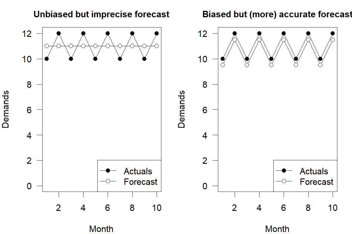
Figure 17.1: Bias vs. accuracy
Let us consider an artificial example (see Figure 17.1). Assume that our point forecast is \((11, 11, \dots, 11)\); that is, we have a constant forecast of \(11\) for \(n = 10\) months. Assume further that the actual observations are \((10, 12, 10, 12, 10, 12, 10, 12, 10, 12)\). Then the errors are \((1, -1, 1, -1, 1, -1, 1, -1, 1, -1)\) and \(\text{ME} = 0\), that is, our flat forecast is unbiased. However, it is inaccurate since \(\text{MAD} = 1\). Conversely, assume that the forecast is \((9.5, 11.5, 9.5, 11.5, \dots, 9.5, 11.5)\). In this case, our errors are \((-0.5, -0.5, \dots, -0.5)\), and every single forecast is \(0.5\) units too low. Therefore, \(\text{ME} = -0.5\), and our forecasts are biased (more precisely, biased downward). However, these forecasts are more accurate than the original ones since their \(\text{MAE} = 0.5\). In other words, even though being unbiased often means a forecast is more accurate, this relationship is not guaranteed. Forecasters sometimes have to decide whether they prefer a biased but more accurate method over an unbiased but less accurate one.
Which of the two forecasts shown in Figure 17.1 is better? We cannot answer this question in isolation. We usually want our forecasts to be unbiased since over- and under-forecasts cancel out in the long run for unbiased forecasts. This logic would favor the first set of forecasts. However, the second set of forecasts better captures the zigzag pattern in the realizations at the expense of bias. To decide which forecast is “better,” we would need to assess which leads to better decisions in plans that depend on the forecast, e.g., which forecast yields lower stocks and out-of-stocks (which in turn depends, in addition to point forecasts, on accurate estimates of future residual variances and on other variables, see Section 17.5).
How strong a bias do our error measures need to exhibit to provide evidence that a forecasting method is indeed biased? After all, it is improbable that the average error is precisely equal to zero. To answer this question, we need to standardize the observed average forecast error by the observed variation in forecast errors – much akin to calculating a test statistic. This standardization is the objective of the tracking signal, which we can calculate as the cumulative sum of errors divided by the Mean Absolute Error:
\[\begin{align} \text{TS} = \frac{\sum \mathit{Error}_i}{\text{MAE}} \tag{17.7} \end{align}\]We constantly monitor the tracking signal. If it falls outside certain boundaries, we deem the forecast biased. A general rule of thumb is that if the tracking signal consistently goes outside the range of \(\pm 4\), that is, if the running sum of forecast errors is four times the average absolute deviation, then this constitutes evidence that the forecasting method has become biased.
One other widespread point forecast accuracy measure often used as an alternative to the MAE, works with squared errors, that is, \(\mathit{Error}^2\). The square turns every negative number into a positive one, so similarly to absolute deviations, squared errors will never be negative. In order to summarize multiple squared errors \(\mathit{Error}_1^2, \dots, \mathit{Error}_n^2\), one can calculate the Mean Squared Error (MSE),
\[\begin{align} \text{MSE} = \frac{1}{n}\sum_{i=1}^n \mathit{Error}_i^2. \tag{17.8} \end{align}\]The MSE is another measure of accuracy, not bias. In the example in the previous section, the first (constant) forecast yields \(\text{MSE} = 1\), whereas the second (zigzag) forecast yields \(\text{MSE} = 0.25\).
Should one use absolute (i.e., MAE) or squared (i.e., MSE) errors to calculate the accuracy of a method? Squared errors have one crucial property: Because of the process of squaring numbers, they emphasize large errors. Indeed, suppose that in the example above, we change a single actual realization from \(10\) to \(20\) without changing the forecasts. Then the MEs change slightly to \(-1\) and \(-1.5\), and the MAEs change slightly to \(1.8\) and \(1.5\), but the MSEs change drastically to \(9\) and \(11.25\).
By squaring errors, the MSE becomes more sensitive to outlier observations than the MAE – which can be a good thing (if outliers are meaningful) or distracting (if you do not want to base your decision-making on outlier observations). If you use the MSE, it is always important to screen forecasts and actuals for large errors and think about what they mean. If these large errors are unimportant in the larger scheme of things, you may want to remove them from the forecast quality calculation or switch to an absolute error measure instead.
In addition, squared errors have one other technical, but fundamental property: Estimating model parameters by minimizing the MSE will always lead to unbiased errors, at least if we understand the underlying distribution well enough. The MAE does not have this property. Optimizing the MAE may lead to systematically biased forecasts, especially when we forecast intermittent or count data – see Section 17.4 and Morlidge (2015) as well as Kolassa (2016a).
Finally, we express squared errors and the MSE in “squared units.” If, for example, the forecast and the actual demand are both defined in dollars, the MSE will be denoted in “squared dollars.” This scale is somewhat unintuitive. One remedy is to take the square root of the MSE to arrive at the Root Mean Squared Error (RMSE) – an error measure similar to a standard deviation and thus somewhat easier to interpret.
17.2 Percentage, scaled and relative errors
All summary measures of error we have considered so far (the ME, MAE/MAD, MSE, and RMSE) have one crucial weakness: They are not scale-independent. If a forecaster tells you that the MAE associated with forecasting a time series with a particular method is 15, you have no idea how good this number is. If the average demand in that series is at about 2,000, an MAE of 15 will imply excellent forecasts! If, however, the average demand in that series is only 30, then an MAE of 15 would be seen as evidence that it is challenging to forecast the series. Thus, without knowing the scale of the series, interpreting any of these measures of bias and accuracy is difficult. One can always use them to compare different methods for the same series (i.e., method 1 has an MAE of 15, and method 2 has an MAE of 10 on the same series; thus, method 2 seems to be better), but any comparison between series becomes challenging.
Typically, we will forecast not a single time series but multiple ones, for example, numerous SKUs, possibly in various locations. Each time series will be on a different order of magnitude. One SKU may sell tens of units per month, while another one may sell thousands. In such cases, the forecast errors will typically be on similar orders of magnitude – tens of units for the first SKU and thousands of units for the second SKU. Thus, if we use a point forecast quality measure like the MAE to decide, say, between different possible forecast algorithms applied to all series, our result will be entirely dominated by the performance of the algorithms on the faster-moving SKU. However, the slower-moving one may well be equally or more important. To address this issue, we will try to express all error summaries on a common scale, which we can then meaningfully summarize in turn. We will consider percentage, scaled and relative errors for this.
Percentage errors
Percentage Errors express errors as a fraction of the corresponding actual demand realization to scale forecast errors according to their time series, that is,
\[\begin{equation} \text{PE} = \frac{\mathit{Error}}{\mathit{Demand}} = \frac{\mathit{Forecast}-\mathit{Demand}}{\mathit{Demand}}. \tag{17.9} \end{equation}\]
We usually express these Percentage Errors as percentages instead of fractions. Thus, a forecast of \(10\) and an actual demand realization of \(8\) will yield a Percentage Error of \(\text{PE} = \frac{10 - 8}{8} = 0.25\), or \(25\%\).
As in the case of unscaled errors in the previous sub-section, the definition we give for Percentage Errors in Equation (17.9) is the most commonly used, but it is not the only one encountered in practice. Some forecasters prefer to divide the error not by the actual but by the forecast (Green and Tashman, 2009). One advantage of this alternative approach is that while the demand can occasionally be zero within the time series (creating a division by zero problem when using demand as a scale), forecasts are less likely to be zero. This modified percentage error otherwise has similar properties as the percentage error defined in Equation (17.9). Note, however, that how we deal with zero demands in the PE calculation can have a major impact on what a “good” forecast is (Kolassa, 2023a), which becomes especially important if we have many zero demands, i.e., when our time series are intermittent (see Section 17.4 below). The same important point as for “simple” errors applies: all definitions have advantages and disadvantages, and it is most important to agree on a standard error measure in a single organization, so we do not compare apples and oranges.
Percentage Errors \(\text{PE}_1 = \frac{\mathit{Error}_1}{\mathit{Demand}_1}, \dots, \text{PE}_n = \frac{\mathit{Error}_n}{\mathit{Demand}_n}\) can be summarized in a similar way as “regular” errors. For instance, the Mean Percentage Error is the simple average of the \(\text{PE}_i\),
\[\begin{align} \text{MPE} = \frac{1}{n}\sum_{i=1}^n\text{PE}_i. \tag{17.10} \end{align}\]The MPE is similar to the ME as a “relative” bias measure. Similarly, we can calculate single Absolute Percentage Errors (APEs),
\[\begin{equation} \begin{split} \text{APE} = \; & |\text{PE}| = \left|\frac{\mathit{Error}}{\mathit{Demand}}\right| \\ = \; & \left|\frac{\mathit{Forecast}-\mathit{Demand}}{\mathit{Demand}}\right| = \frac{\left|\mathit{Forecast}-\mathit{Demand}\right|}{\mathit{Demand}}. \end{split} \tag{17.11} \end{equation}\]
where one assumes \(\mathit{Demand}>0\). APEs can then be summarized by averaging to arrive at the Mean Absolute Percentage Error (MAPE),
\[\begin{align} \text{MAPE} = \frac{1}{n}\sum_{i=1}^n|\text{PE}_i| = \frac{1}{n}\sum_{i=1}^n\text{APE}_i. \tag{17.12} \end{align}\]which is an extremely common point forecast accuracy measure – but is more dangerous than it looks (Kolassa, 2017).
Let us look closer at the definition of percentage errors. First, note that percentage errors are asymmetric. If we exchange the forecast and the actual demand, the error switches its sign, but the absolute and squared errors do not change. In contrast, the percentage error changes in a way that depends on the forecast and the demand if we exchange the two. For instance, a forecast of \(10\) and a demand of \(8\) yield \(\text{PE} = 0.25 = 25\%\), but a forecast of \(8\) and a demand of \(10\) yield \(\text{PE} = 0.20 = 20\%\). The absolute error is \(2\), and the squared error is \(4\) in either case.
Second, if the demand is zero, then calculating the APE entails a division by zero, which is mathematically undefined; i.e., if the actual realization is zero, then any non-zero error is an infinite fraction of it. There are various ways of dealing with the division by zero problem (Kolassa, 2023a).
Some forecasting software “deals” with the problem by sweeping it under the rug: in calculating the MAPE, it only sums \(\text{PE}_i\)s whose corresponding actual demands are greater than zero (Hoover, 2006). This approach is not a good way of addressing the issue. It amounts to positing that we do not care at all about the forecast if the actual demand is zero. If we make production decisions based on the forecast, then it will matter a lot whether our prediction was \(100\) or \(1000\) for an actual demand of zero – and such a difference should be reflected in the forecast accuracy measure.
An alternative, which also addresses the asymmetry of percentage errors noted above, is to “symmetrize” the percentage errors by dividing the error not by the actual but by the average of the forecast and the actual (Makridakis, 1993), yielding a Symmetric Percentage Error (SPE),
\[\begin{align} \text{SPE} = \frac{\mathit{Forecast}-\mathit{Demand}}{\frac{1}{2}(\mathit{Forecast}+\mathit{Demand})}. \tag{17.13} \end{align}\]and then summarizing the absolute values of these symmetric percentage errors as usual, yielding a symmetric MAPE (sMAPE),
\[\begin{align} \text{sMAPE} = \frac{1}{n}\sum_{i=1}^n|\text{SPE}_i|. \tag{17.14} \end{align}\]Assuming that at least one forecast and the actual demand are positive, the symmetric error is well defined, and calculating the sMAPE poses no mathematical problems. In addition, the symmetric error is symmetric: if we exchange the forecast and the actual demand, then the symmetric error changes its sign, but its absolute value remains unchanged.
Unfortunately, some problems remain with this error definition. While the symmetric error is symmetric under the exchange of forecasts and actuals, it introduces a new kind of asymmetry (Goodwin and Lawton, 1999). If the actual demand is \(10\), forecasts of \(9\) and \(11\) (an under- and over-forecast of one unit, respectively) result in APEs of \(0.10 = 10\%\). However, a forecast of \(9\) yields an SPE of \(\frac{-1}{9.5}\approx-0.105 = -10.5\%\), whereas a forecast of \(11\) yields an SPE of \(\frac{1}{10.5} \approx 0.095 = 9.5\%\). Generally, an under-forecast by a given difference will yield a larger absolute SPE than an over-forecast by the same amount, whereas the APE will be the same in both cases.
And this asymmetry is not the last of our worries. As noted above, using the SPE instead of the PE means we can mathematically calculate an SPE even when the demand is zero. However, what acually happens for the SPE in this case? Let us calculate:
\[\begin{align} \text{SPE} = \frac{\mathit{Forecast}-\mathit{Demand}}{\frac{1}{2}(\mathit{Forecast}+\mathit{Demand})} = \frac{\mathit{Forecast}-0}{\frac{1}{2}(\mathit{Forecast}+0)} = 2 = 200\%. \end{align}\]Thus, whenever actual demand is zero, the symmetric error SPE contributes 200% to the sMAPE, entirely regardless of the forecast (Boylan and Syntetos, 2006). Dealing with zero demand observations this way is not much better than simply disregarding errors whenever actual demand is zero, as above.
Finally, we can calculate a percentage summary of errors differently to address the division by zero problem. We define the weighted MAPE (wMAPE) as
\[\begin{align} \text{wMAPE} = \frac{\sum_{i=1}^n|\mathit{Error}_i|}{\sum_{i=1}^n\mathit{Demand}_i} = \frac{\text{MAE}}{\mathit{Mean~Demand}}. \tag{17.15} \end{align}\]A simple computation (Kolassa and Schütz, 2007) shows that we can interpret the wMAPE as a weighted average of APEs if all demands are positive, where the corresponding demand weights each \(\text{APE}_i\). In the wMAPE, a given APE has a higher weight if the related realization is larger, which makes intuitive sense. In addition, the wMAPE is mathematically defined even if some demands are \(0\), as long as not all demands are \(0\).
Interpreting wMAPE as a weighted average APE, with weights corresponding to actual demands, suggests alternative weighting schemes. After all, while the actual demand is one possible measure of the “importance” of one APE, there are other possibilities for assigning “importance” to an APE, like the cost of an SKU or its margin. As mentioned above, agreeing on a single standard way of calculating the wMAPE within an organization is vital.
Apart from the problem with dividing by zero, which we can in principle address by using the wMAPE, the MAPE unfortunately has another issue that does not necessarily invalidate its use but that we should keep in mind. The \(\text{PE}\)s can become very large if the demand is small, even if all demands are above zero. Thus, the APEs for small demands will dominate the MAPE calculation, which incentivizes us to bias our forecast downward.
A helpful way of looking at this is to consider the MAPE as a weighted sum of AEs, with weights that are given as the reciprocal of observed demands:
\[\begin{equation} \begin{split} \text{MAPE} =\;& \frac{1}{n}\sum_{i=1}^n\text{APE}_i = \frac{1}{n}\sum_{i=1}^n \frac{\left|\mathit{Forecast}_i-\mathit{Demand}_i\right|}{\mathit{Demand}_i} \\ =\;& \frac{1}{n}\sum_{i=1}^n \frac{1}{\mathit{Demand}_i}\times\left|\mathit{Forecast}_i-\mathit{Demand}_i\right| \\ =\;& \frac{1}{n}\sum_{i=1}^n \frac{1}{\mathit{Demand}_i}\times\text{AE}_i. \end{split}\tag{17.16} \end{equation}\]We see that the same AE will get a higher weight in the MAPE calculation if the corresponding demand is smaller. Minimizing the MAPE thus drives us toward reducing the AEs in particular on smaller demands – which will usually mean reducing all forecasts, i.e., biasing our forecasts downward.
| Low Forecast | High Forecast | |
|---|---|---|
| Low actual | APE is zero | APE is high |
| High actual | APE is low | APE is zero |
As an illustration, assume our demand has only two possible values, low and high, and that we can also only forecast “low” or “high” (see Table 17.1). If we forecast “low” and demand is low, we have a zero error, and a zero APE. The same holds if we forecast “high” and demand also turns out to be high. Things become more interesting if we forecast wrong. Irrespective of the direction of our error, the AE is the same, i.e., the difference between the high and the low value. What changes between these two possible situations is the weight given to this AE. If we forecast “low” and demand is high, we weight the AE by the reciprocal of the high value, so we get a low APE. But if we forecast “high” and the demand is low, our weight is the reciprocal of a low value, so the APE will be high! Minimizing means forecasting low.
Kolassa and Martin (2011) give a simple illustration of a similar effect that you can try at home. Take any standard six-sided die and forecast its roll. Assuming the die is not loaded, all six numbers from one to six are equally likely, and the average roll is \(3.5\). Thus, an unbiased forecast would also be \(3.5\). What MAPE would we expect from forecasting \(3.5\) for a series of many die rolls? We can simulate this expected MAPE empirically by rolling a die many times. Alternatively, we can calculate it abstractly by noting that we have one chance in six in rolling a one, with an APE of \(|1-3.5|/1 = 250\%\), another one-in-six chance of rolling a two, with an APE of \(|2-3.5|/2 = 75\%\), and so on. It turns out that our expected MAPE is 71% for a forecast of 3.5.
We can use our dice to see what happens if we use a biased forecast of \(4\) instead of an unbiased forecast of \(3.5\). Little surprise here – the long-run MAPE of a forecast of \(4\) is worse than for a forecast of \(3.5\): it is 81%. However, what happens if our forecast is biased low instead of high? This time, we are in for a surprise: a forecast of \(3\) yields an expected MAPE of 61%, clearly lower than the MAPE for an unbiased forecast of \(3.5\). And an even more biased forecast of \(2\) results in a yet lower long-run MAPE of 52%. Try this with your dice at home!
Explaining this effect requires understanding the asymmetry of MAPE. Any forecast higher than \(2\) will frequently result in an APE larger than 100%, for example, if we roll a one. Such high APEs pull the average up more than lower APEs can pull it down. The bottom line is that the expected MAPE is minimized by a forecast that is heavily biased downward. Using this KPI can then lead to very dysfunctional incentives in forecasting.
Interestingly, this simple example shows that alternatives to “vanilla” MAPE, such as the sMAPE or the MAPE with the forecast as a denominator, are also minimized by forecasts that differ from the actual long-run average. This asymmetry in the APE creates a perverse incentive to calculate a biased low forecast rather than one that is unbiased but has a chance of exceeding the actual by a factor of \(2\) or more (resulting in an APE \(> 100\%\)). These incentives could tempt a statistically savvy forecaster to apply a “fudge factor” to the statistical forecasts obtained using their software, reducing all system-generated forecasts by (say) 10%.
Scaled errors
An alternative to using percentage errors is calculating Scaled Errors, where we scale the MAE/MAD, MSE, or RMSE (or any other error measure) by an appropriate amount. One scaled error measure is the Mean Absolute Scaled Error (Franses, 2016; Hyndman, 2006; MASE; see Hyndman and Koehler, 2006). Its computation involves not only forecasts and actual realizations, but also historical observations used to calculate forecasts, because the scaling factor used is the MAE of the naive forecast in-sample.
Specifically, assume that we have historical observations \(y_1, \dots, y_T\), from which we calculate one-step-ahead, two-step-ahead, and later forecasts \(\hat{y}_{T+1}, \dots, \hat{y}_{T+h}\), which correspond to actual realizations \(y_{T+1}, \dots, y_{T+h}\). Using this notation, we can write our MAE calculations as follows:
\[\begin{align} \text{MAE} = \frac{|\hat{y}_{T+1}-y_{T+1}|+\dots+|\hat{y}_{T+h}-y_{T+h}|}{h}. \tag{17.17} \end{align}\]To define a scaling factor for this MAE, we calculate the MAE that we would have observed if we had used naive one-step-ahead forecasts in the past. That is, simply using the previous demand observation to forecast the future. The naive one-step forecast for period 2 is the previous demand \(y_1\), for period 3 the previous demand \(y_2\), and so forth. Specifically, we calculate
\[\begin{align} \text{MAE}' = \frac{|y_1-y_2| + \dots + |y_{T-1}-y_T|}{T-1}. \tag{17.18} \end{align}\]The MASE then is the ratio of \(\text{MAE}\) and \(\text{MAE}'\):
\[\begin{align} \text{MASE} = \frac{\text{MAE}}{\text{MAE}'}. \tag{17.19} \end{align}\]The \(\text{MASE}\) thus scales \(\text{MAE}\) by \(\text{MAE}'\). It expresses whether our “real” forecast error (MAE) is larger than the in-sample naive one-step ahead forecast (\(\text{MASE} > 1\)) or smaller (\(\text{MASE} < 1\)). Since the numerator and denominator are on the scale of the original time series, we can compare the MASE between different time series.
Keep two points in mind. First, the MASE is often miscalculated. The correct calculation requires using the in-sample, naive forecast for \(\text{MAE}'\), that is, basing the calculations on historical data used to estimate the parameters of a forecasting method. Instead, forecasters often use the out-of-sample, naive forecast to calculate \(\text{MAE}'\), that is, the data to which the forecasting method is applied. This miscalculation also results in a defensible scaled forecast quality measure. Still, it is not “the” MASE as defined in literature (Hyndman and Koehler (2006) give a technical reason for proposing the in-sample MAE as the denominator). As always, one just needs to be consistent in calculating, reporting, and comparing errors in an organization.
Second, as discussed above, a \(\text{MASE} > 1\) means our forecasts have a worse MAE than an in-sample, naive, one-step-ahead forecast. This, at first glance, sounds disconcerting. Should we not expect to do better than the naive forecast? However, a \(\text{MASE} > 1\) could easily come about using quite sophisticated and competitive forecasting algorithms (e.g., Athanasopoulos et al., 2011 who found \(\text{MASE} = 1.38\) for monthly, \(1.43\) for quarterly, and \(2.28\) for yearly data). For instance, remember that we potentially calculate the MASE numerator’s MAE from multi-step-ahead forecasts. In contrast, we calculate the \(\text{MAE}'\) in the denominator from one-step-ahead forecasts. It is not surprising that multi-step-ahead forecasts are worse than one-step-ahead (naive) forecasts.
What are the advantages of the MASE compared to the MAPE? First, it is scaled, so the MASE of forecasts for time series on different scales is comparable. This attribute is similar to MAPE. However, the MASE has two critical advantages over MAPE. First, it is defined even when one demand realization is zero. Second, it penalizes AEs for low and high actuals equally, avoiding the problem we encountered in the dice-rolling example. On the other hand, MASE does have the disadvantage of being harder to interpret. A percentage error (as for MAPE) is easier to understand than a scaled error as a multiple of some in-sample forecast (as for MASE).
Relative errors
Yet another variation on the theme of error measures is given by Relative Errors. We can calculate relative errors for any underlying error measure, e.g., those we considered above and those we will consider in Section 17.3. They always work relative to some benchmark forecast or forecasting method. Essentially, relative errors answer the question of whether and by how much a given focal forecast is better than some benchmark forecast, as measured by the chosen error measure.
For example, assume we use the naive forecast as the benchmark and decide to use the MSE as an error measure. Assume that the benchmark naive forecast yields an MSE of 10 on a holdout dataset. We now fit our favorite model, calculate forecasts on the same holdout data, and again evaluate the MSE of this forecast. Let us assume that this MSE is 8. Then the relative MSE, often abbreviated relMSE (“RMSE” could cause confusion with the Root Mean Squared Error) is
\[\begin{align} \text{relMSE} = \frac{\text{MSE}_{\text{focal forecast}}}{\text{MSE}_{\text{benchmark forecast}}} = \frac{8}{10} = 0.8. \end{align}\]Thus, a \(\text{relMSE} < 1\) indicates that our focal forecast performs better than the benchmark, and \(\text{relMSE}>1\) suggests that it performs worse, both in terms of the MSE. Per Chapter 8, it always makes sense to consider simple forecasting methods as benchmarks, and relative errors give us a tool to do so: calculate the relative error of your focal forecast against the historical mean or the naive forecast, using whatever error measure you want.
One disadvantage of relative errors is that they only give relative information. Suppose you calculate the relative MAE of a forecast with respect to the naive forecast. In that case, you will learn how much smaller your focal forecast’s MAE is than the naive forecast’s in relative terms, but you will not know anything in absolute terms. Based on relative measures alone, we can only say whether a focal forecast is better than a benchmark, but not by how much in absolute terms nor how good the benchmark forecast was itself.
17.3 Assessing prediction intervals and predictive distributions
Recall from Section 4.2 that a prediction interval for a given coverage level (e.g., 80%) consists of a lower and an upper quantile forecast of future demand such that we expect a corresponding percentage of 80% of future realizations to fall between the quantile forecasts. How do we assess whether such an interval forecast is any good?
A single interval forecast and a corresponding single demand realization do not yield much information. Even if the prediction interval captures the corresponding interval of the underlying probability distribution perfectly (which is referred to as perfectly calibrated), then the prediction interval is expected not to contain the actual realization in one out of every five cases in our example with a target coverage proportion of 80%. If we observe just a few instances, we can learn little about the accuracy of our method of creating prediction intervals. An assessment of calibration requires larger amounts of data.
Furthermore, the successful assessment of prediction intervals requires that we fix the method of creating these intervals over time. Suppose we want to examine whether the prediction intervals provided by a forecaster are 80%; if we allow changing the method of creating prediction intervals between observations, the forecaster could simply set vast intervals for four of these periods (being almost certain to contain the observation) and a very narrow interval for the remaining period (which will probably not contain the observation), creating an 80% “hit rate.” Needless to say, such gamed prediction intervals are of little use.
In summary, to assess the calibration of prediction interval forecasts, we will need multiple demand observations from a time period when the method used to create these intervals was fixed. Suppose we have \(n\) interval forecasts and that \(k\) of them contain the corresponding demand realization. We can then compute the achieved coverage rate \(\frac{k}{n}\) and compare it to the target coverage rate \(q\). Our interval forecast looks good if \(\frac{k}{n} \approx q\). However, we will usually not exactly have \(\frac{k}{n} = q\). Thus, the question arises of how large the difference between \(\frac{k}{n}\) and \(q\) must be to reasonably conclude that our method of constructing interval forecasts is good or bad. We can use a statistical concept called “Pearson’s \(\chi^2\) test.” We create a so-called contingency table by noting how often our interval forecasts covered the realization and how often we would have expected them to do so: see Table 17.2 for this table.
| Covered | Not Covered | |
|---|---|---|
| Observed | \(k\) | \(n-k\) |
| Expected | \(qn\) | \((1-q)n\) |
We next calculate the following test statistic:
\[\begin{align} \chi^2 = \frac{(k-qn)^2}{qn} + \frac{\big(n-k-(1-q)n\big)^2}{(1-q)n}. \tag{17.20} \end{align}\]The symbol “\(\chi\)” represents the small Greek letter “chi,” and this test is therefore often called a “chi-squared” test. We can then examine whether this calculated value is larger than the critical value of a \(\chi^2\) distribution with one degree of freedom for a given \(\alpha\) (i.e., statistical significance) level. This critical value is available in standard statistical tables or software, for example, using the =CHISQ.INV function in Microsoft Excel. Suppose our calculated value from Equation (17.20) is larger than the critical value. In that case, we have evidence of poor calibration, and we should consider improving our method of calculating prediction intervals.
For example, let us assume we have \(n = 100\) interval forecasts aiming at a nominal coverage probability of \(q = 95\%\), so we would expect \(qn = 95\) of actual realizations to be covered by the corresponding interval forecasts. Let us assume we observe \(k = 90\) realizations covered by the interval forecast. Is this difference between observing \(k = 90\) and expecting \(qn = 95\) covered realizations statistically significant at a standard alpha level of \(\alpha = 0.05\)? We calculate a test statistic of
\[\begin{align} \chi^2=\frac{(90-95)^2}{95} + \frac{(10-5)^2}{5} = 0.26 + 5.00 = 5.26. \end{align}\]The critical value of a \(\chi^2\) distribution with 1 degree of freedom for an \(\alpha = 0.05\), calculated for example using Microsoft Excel by =CHISQ.INV(0.95;1), is \(3.84\), which is smaller than our test statistic. We conclude that our actual coverage is statistically significantly smaller than the nominal coverage we had aimed for and thus consider modifying our way of calculating prediction intervals.
In addition, there are more sophisticated (but also more complex) methods of evaluating prediction intervals, like the interval score – see Section 2.12.2 in Petropoulos, Apiletti, et al. (2022) for a discussion. An alternative is to not assess the prediction interval as such, but to evaluate the two endpoints separately, treating them as two separate quantile forecasts. The method of choice for this is the pinball loss (Kolassa, 2023b) and its variants. For instance, the M5 competition used a scaled version of the pinball loss to make it comparable across series on different aggregation levels (Makridakis, Spiliotis, Assimakopoulos, Chen, et al., 2022).
Finally, we have discussed that the most informative forecast is a full predictive distribution. How would we evaluate this? The tools for this are so-called proper scoring rules, which are unfortunately highly abstract and very hard to interpret. See Section 2.12.4 in Petropoulos, Apiletti, et al. (2022) for a discussion and examples.
17.4 Accuracy measures for count data forecasts
Count data, unfortunately, pose particular challenges for forecast quality assessments. Some quality measures investigated so far can be seriously misleading for count data. For instance, the MAE does not work as expected for count data (Kolassa, 2016a; Morlidge, 2015). The underlying reason is well known in statistics, but you will still find forecasting researchers and practitioners incorrectly measuring the quality of intermittent demand forecasts using the MAE.
What is the problem with MAE and count data? There are two key insights that can help us understand this issue. One is that we want a point forecast quality measure to guide us toward unbiased point forecasts. Put differently, we want any error measure to have a minimum on average if we feed it unbiased forecasts. Unfortunately, the MAE does not conform to this requirement. Whereas the MSE is minimized and the ME is zero in expectation for an unbiased forecast, the MAE is not minimized by an unbiased forecast for count data. Specifically, the forecast that minimizes the expected (mean) absolute error for any distribution is not the expected value of a distribution but its median (Hanley et al., 2001). This fact does not make a difference for a symmetric predictive distribution like the normal distribution, since the mean and the median of a symmetric distribution are identical. However, the distributions we use for count data are hardly ever symmetric, and this deficiency of the MAE thus becomes troubling – and potentially disastrous.
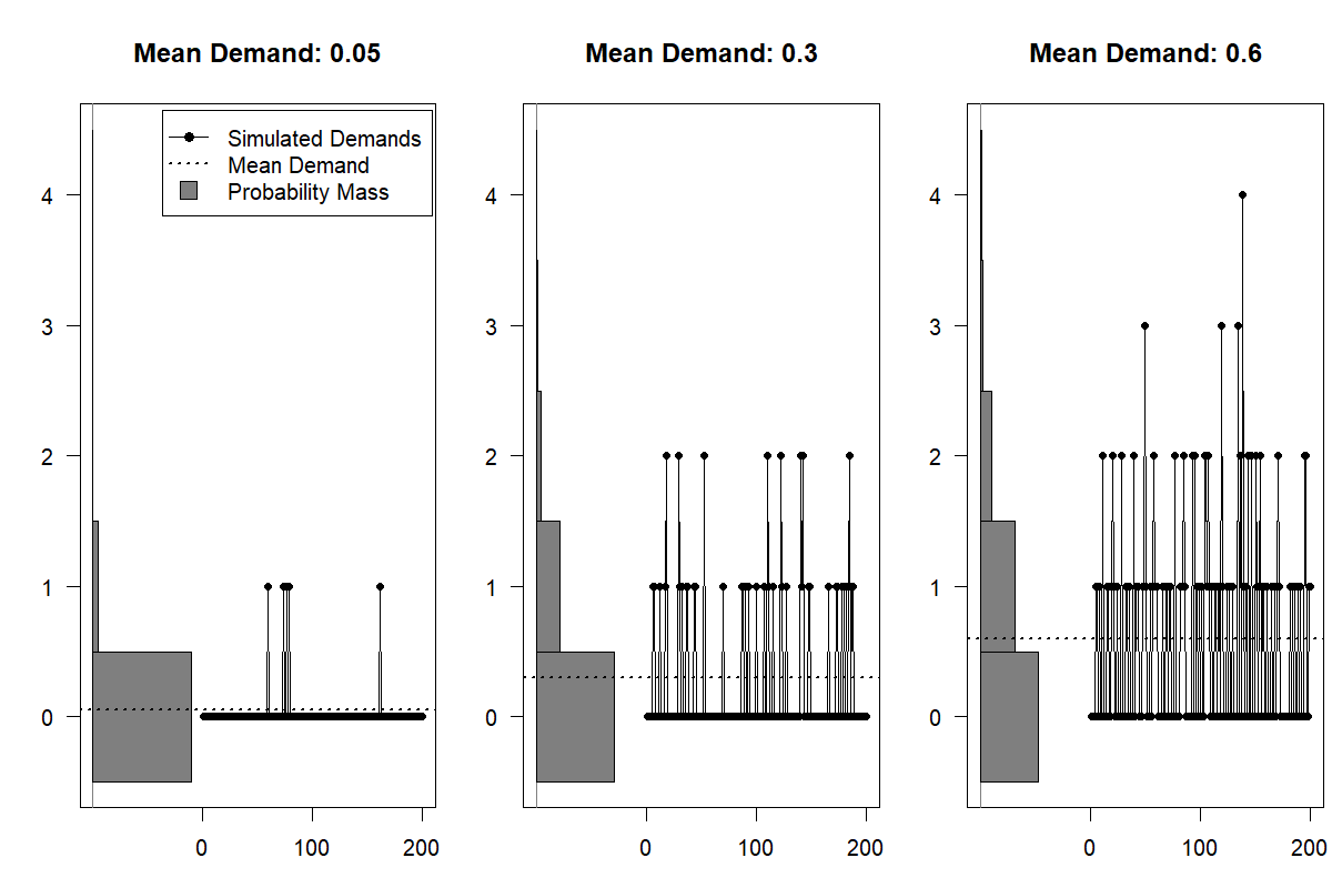
Figure 17.2: Poisson-distributed count demand data
As an example, Figure 17.2 shows three Poisson-distributed demand series with different means (\(0.05\), \(0.3\), and \(0.6\)), along with probability mass histograms turned sideways. Importantly, in all three cases, the median of the Poisson distribution is zero, meaning that the point forecast that minimizes the MAE is zero.
Turning this argument around, suppose we use the MAE to find the “best” forecasting algorithm for several count data series. We find that a flat zero-point forecast minimizes the MAE. This is not surprising after our prior discussion. However, a flat zero forecast is not useful. The inescapable conclusion is that we need to be very careful about using the MAE for assessing point forecasts for count data!
Unfortunately, this realization implies that all point forecast quality measures that are only scaled multiples of the MAE are equally useless for count data. Specifically, this applies to the MASE and the wMAPE.
Finally, the MAPE does not make any sense for intermittent data since the APE is undefined if the actual is zero (Kolassa, 2017). There have been many proposals on dealing with this issue, as discussed above. It turns out that how exactly we deal with zero actuals in the context of the MAPE has a significant impact on what the best forecast (in terms of minimizing the expected MAPE) for a given time series is and on the sheer scale of the MAPE we can expect (Kolassa, 2023a). Of course, this problem is more prevalent the more intermittent the time series is.
Some quality measures do work as expected for count data. The ME is still a valid measure of bias. However, highly intermittent demands can, simply by chance, have long strings of consecutive zero demands so that any non-zero forecast may look biased. Thus, detecting bias is even harder for count data than for continuous data. Similarly, the MSE retains its property of being minimized by the expectation of future realizations. Therefore, we can still use the MSE to guide us toward unbiased forecasts. However, as discussed above, the MSE can still not be meaningfully compared between time series of different levels, so scaled errors are just as relevant for intermittent series as for non-intermittent ones.
17.5 Forecast accuracy and business value
Forecasters regularly evaluate the quality of their forecasts using error measures described in the previous sections. However, these measures consider just one aspect of the quality of the forecast produced: the error of the forecast compared to the actual outcome. A forecast does not exist for its own purpose. The purpose of forecasting is not to provide the best forecast, but to enable the best decision that is informed by the forecast. Common error measures fail to consider the forecast’s usefulness in making better decisions. Thus, they are insufficient to evaluate the ultimate value of a forecasting method (Yardley and Petropoulos, 2021).
Although the forecast plays a key role in the decision-making process, it is not the only input. Other elements also have to be considered, often in the form of costs, capacities, constraints, policies and business rules. A number of research projects have demonstrated that the efficiency of the decision-making processes does not relate directly to demand forecasting performance, as measured by standard error measures (Syntetos et al., 2010). The fact that forecasting method A performs better than forecasting method B in terms of error measures (however this is measured) does not necessarily imply that method A will lead to better decisions than B (Robette, 2023).
Better forecasts won’t earn you money. Better production plans, capacity utilization, or stock control will. The best forecast is not the perfect forecast, or the one with the highest accuracy or lowest error, but the one that allows the best decisions to be made. Forecast accuracy is only a means to an end. And yes, this implies that interpreting forecast accuracy without looking at the larger picture is short-sighted. The mission of forecasters should therefore not be to minimize the error between a forecast and reality, but to maximize the business benefit. (This is why we believe that forecasters also need to understand the larger picture, and to have good communication skills for the necessary cross-functional discussions, see Section 19.1).
When evaluating the quality of a forecast, we thus need to measure the implications of different forecasts. Forecasts generated by method A may be more accurate than forecasts generated by method B, but if subsequent processes mean that they have the same implications (e.g., because we are using forecasts as an input to a production planning process, but logistical constraints mean that both forecasts will lead to the same production plan), then in terms of actual outcomes, both forecasts are equally good.
One way to investigate this is by simulating the processes that turn forecasts into decisions (Kolassa, 2023b). Such a simulation is usually not easy, since the following processes are complicated. However, setting up such a simulation, making reasonable simplifications, is often much more enlightening than chasing forecast accuracy improvements without knowing whether they actually translate into business value.
Key takeaways
- There are numerous forecast accuracy measures.
- Different accuracy measures measure different things. There is no one “best” accuracy KPI. Consider looking at multiple ones, but be aware that different KPIs reward different forecasts.
- If you have only a single time series or series on similar scales, use MSE or MAE.
- Use scaled or percentage errors if you have multiple series at different scales. However, remember that these percentage errors can introduce asymmetries concerning how they penalize over- and under-forecasting.
- Always look at bias. MAE and MAPE can mislead you into biased forecasts, especially for low-volume series.
- You get what you reward, so choose error metrics that are aligned with the business outcome. Be aware that there is much scope for gaming poorly chosen error metrics, by human forecasters or forecasting tools and models.
- Forecast accuracy is not necessarily the same as business value. Beware of chasing worthless accuracy improvements.