15 Long, multiple and non-periodic seasonal cycles
Previous chapters discussed incorporating simple forms of seasonality – e.g., the yearly seasonality for quarterly or monthly data – into our models. The present chapter will consider challenges posed by “more complicated” seasonality. The workhorses of forecasting, i.e., Exponential Smoothing and ARIMA, were developed when time series were primarily monthly or quarterly. Today, we collect time series data at a far higher frequency, e.g., daily or hourly. This increased granularity can yield more complicated seasonal patterns. Exponential Smoothing and ARIMA models may not be able to deal with such seasonality.
15.1 Introduction
The first thing to be aware of when we examine more complicated seasonality is that when we discuss seasonality, we always have to know two pieces of time-related information: the temporal granularity of our time buckets, and the cycle length at which patterns repeat seasonally. For instance, we could have a daily granularity and a weekly cycle, meaning that demands on Mondays are similar to each other, also on Tuesdays and so on. However, we might also have hourly granularity and a daily cycle, in which case the hourly demand at 9:00 a.m. is similar between different days. We see that “daily” here crops up in two different places: either as the granularity, or as the cycle length. A term like “daily seasonality” is ambiguous: does it refer to sub-daily time buckets (e.g., hourly) with a daily cycle, or to daily buckets with a cycle that comprises multiple days (e.g., a weekly, monthly, or yearly cycle)? “Monthly seasonality” could similarly refer to daily data with patterns that repeat every month (like payday effects), or monthly data with recurring patterns every 3 months (quarterly cycles) or every 12 months (yearly cycles).
| Granularity | Cycle (buckets per cycle) | Examples |
|---|---|---|
| Quarter hour | Day (96 buckets) | Call center demand,Electricity demand |
| Hour | Day (24 buckets) | Traffic flow |
| NA | NA | Residential water demand |
| Day | Week (7 buckets) | Retail demand |
| Day | 2 Weeks (14 buckets) | US paycheck effects |
| Day | Month (28-31 buckets) | German paycheck effects |
| Day | Year (About 365 buckets) | Gardening supplies |
| Week | Year (About 52 buckets) | Gardening supplies |
| Month | (About 12 buckets) | Ice cream demand |
Often, what is meant is clear from the context – if our time series are all on daily granularity, then “monthly seasonality” probably refers to patterns of demand that recur every 28-31 days. However, especially if we are talking to someone with a different background, where misunderstandings can easily happen, it makes sense to be as clear as possible and explicitly say what we are thinking of: “daily data with monthly seasonality.” Table 15.1 gives a few examples of possible granularity-cycle combinations.
Figure 15.1 summarizes the different ways in which seasonality can become more complicated than previously discussed:
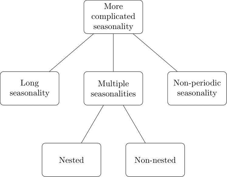
Figure 15.1: An overview of more complicated seasonality
Long seasonality occurs if a seasonal cycle involves many time buckets. For instance, consider the call volume on a weekday per \(15\)-minute time bucket at a call center that works 24 hours. We can divide each weekday into \(4\times 24=96\) periods per daily cycle. If the call center also works on weekends, we will likely have multiple seasonalities; see below. We discuss ways to address long seasonality in Section 15.2.
The term “long seasonality” refers to having many time buckets within a seasonal cycle and does not imply having a long data history. A decade-long time series of quarterly data (4 periods per annual cycle) is not long seasonality. Hourly data with daily seasonality (24 hours a day) border on long seasonality, and longer seasonal periods are clearly so, like 28 to 31 days a month, 96 quarter-hourly buckets in a day, or 168 hours in a week.
If our demand series exhibits layers of seasonal cycles of different lengths, we refer to multiple seasonalities. An example might be hourly website traffic, where the daily pattern differs by the day of the week. In other words, we have a daily cycle of length 24 and a weekly cycle of length \(7\times 24 = 168\).
In this particular example, the seasonalities are nested within each other: the longer seasonal cycle (168 hours) contains multiple entire shorter seasonal cycles (7 days of 24 hours each). We can also have non-nested multiple seasonalities. For example, daily data may have a weekly (i.e., week of the year) and a monthly pattern. Some weeks fall into two months, so weeks are not nested within months. We discuss multiple seasonalities in Section 15.3 and give a more detailed example in Section 15.4.
Multiple seasonalities usually imply long seasonality but not vice versa. In the example of 15-minute weekday demand at a call center, we have long daily seasonality with \(96\) periods per cycle. But there is, per se, no other seasonal cycle involved.
Non-periodic seasonality refers to patterns with periodicities that do not align with the standard western calendar or have changing period lengths. Most examples stem from religious or cultural events driven by the lunar calendar, like Easter, Jewish or Islamic holidays, or the Chinese New Year. A more prosaic example is a payday effect if paychecks arrive monthly: the cycle length varies between 28 and 31 days and is thus irregular.
We discuss ways of modeling all three kinds of complicated seasonality in Sections 15.5 and 15.6.
15.2 Long seasonality
Exponential Smoothing and ARIMA models suffer from estimation issues with long seasonality. For instance, Exponential Smoothing must estimate one starting parameter value for each time bucket in a seasonal cycle. It is easy to estimate \(12\) monthly indices for yearly seasonality, but far more challenging to estimate \(168\) hourly indices for weekly seasonality. Not only does the numerical estimation take time, but the high number of parameters involved creates model complexity, which can lead to a noisy, unstable, and poorly performing model (see Section 11.7).
Good software design will prevent you from estimating overly complex models by refusing to model long seasonalities in this way. For example, the ets() function in the forecast package for R will only allow seasonal cycles of lengths up to \(24\), i.e., hourly data with daily seasonality. If you try to model longer seasonal cycles, the software will suggest using an STL decomposition instead – one of our recommendations below.
15.3 Multiple seasonalities
Data collection happens on ever-finer temporal granularity. This results in time series that exhibit multiple seasonal cycles of different lengths. For instance, hourly demand data can reveal intra-daily and intra-weekly patterns, and hourly supermarket ice cream sales will show intra-daily and intra-yearly seasonality. Cycles can be nested within each other (e.g., hours within days within months within years) or are non-nested (e.g., weeks within months). They can also change over time. Practical examples with multiple seasonalities include electricity load demand, emergency medicine demand, hospital admissions, call center demand, public transportation demand, traffic flows, pedestrian counts, requests for cash at ATMs, water usage, or website traffic.
Hypothesizing such complicated patterns alone does not always warrant including them in our models. We can examine whether the underlying signal is strong enough to warrant more complex models through (possibly adapted) seasonal plots (see, for example, Figure 15.4). Researchers and practitioners have developed several new (and more complex) approaches to modeling multiple seasonalities. Recall from Section 11.7 that complex models are not always better. Don’t be surprised if they don’t outperform simpler approaches.
15.4 An example: ambulance demand
An example of multiple seasonalities is emergency medical services. To illustrate, we examine a time series of ambulance demand data from a large ambulance service in the United Kingdom. The dataset contains the hourly number of ambulances demanded (or similar incidents). Figure 15.2 shows the daily ambulance demand plotted for \(5\) years. It is challenging to identify patterns, given the sheer number of data points plotted.
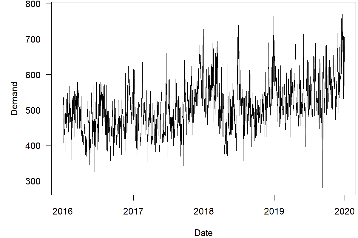
Figure 15.2: Daily time series of ambulance demand
Figure 15.3 graphs two weeks of hourly ambulance demand. The regular intra-daily pattern is evident in this plot. The cycles for Monday through Sunday look similar.
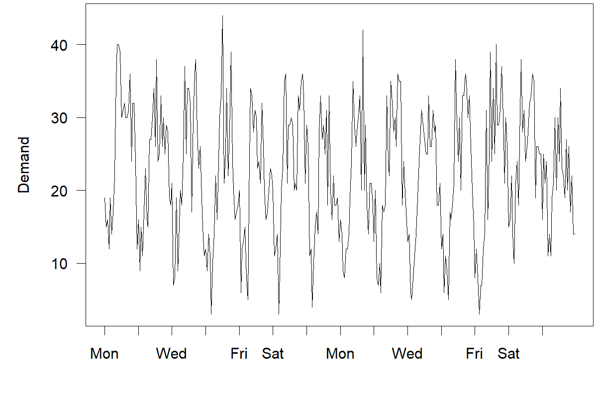
Figure 15.3: A two week sample of hourly ambulance demand
Figure 15.4 depicts a seasonal plot of the average number of incidents per hour separately for each day of the week, from January 2016 to December 2019. Ambulance demand follows an apparent intra-daily pattern. It decreases between midnight and early morning and then increases until the evening, decreasing again until midnight. The changes in the ambulance demand per hour of the day reflect the population’s activities, such as driving, working, hiking, etc. As the number of activities increases during the daytime, we see more people requesting ambulances.
Intra-weekly effects are also visible. People demand more ambulances on Monday and fewer ones on Sunday. This pattern again likely reflects the distribution of human activity throughout the week. Events like weekends, nights out, festivals, rugby matches, etc. shift the place of activities and change the demand for ambulance services. Demand is also higher on Saturday and Sunday between midnight and 5 a.m. This shift also holds for Friday and Saturday between 7 p.m. and midnight. These demand shifts originate from the temporal distribution of human activities and behaviors.
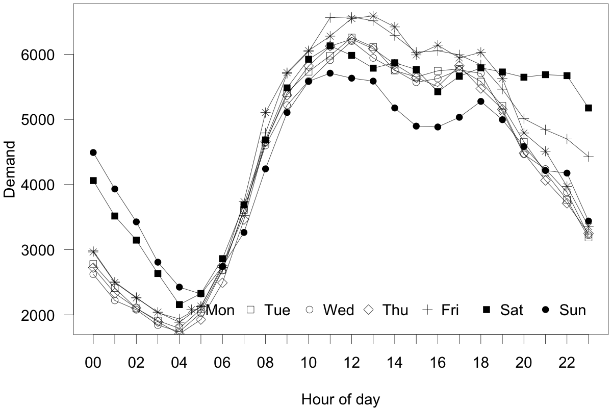
Figure 15.4: Average ambulance demand per hour, seperated by the day of the week
15.5 Modeling complicated seasonality
There are four main ways to account for long, multiple, or non-periodic seasonalities in time series forecasting. We can model such seasonality using predictors, lagged terms, seasonal dummy variables, or harmonics.
Predictors
Seasonality has an underlying cause. If we know the drivers of seasonality and if we can measure and forecast them, we can use these measures to model and explain seasonal variation in our time series data. For example, suppose that our firm schedules a product promotion every two weeks. To capture this behavior using seasonality, we would have to deal with the issue of not every month having the same number of weeks. The model would get complicated. But if we can measure whether a promotion occurs, we do not need to model this seasonality; instead, we can simply add this single predictor to your model.
We discuss using predictors in forecasting in Chapter 11. If we can identify predictors that describe or are associated with the seasonal patterns in our time series data, we should include them in the model. We should also investigate each predictor’s potential lagged relationship structure (see also Section 11.3).
It can be challenging to measure these predictors over time consistently. Depending on how we use them in our models, we may need to forecast them, reducing their accuracy. For example, if we use temperature as a predictor, we will not know the future temperature. We would need temperature forecasts, which creates an extra layer of uncertainty. If the association between predictors and the forecast variable is weak, or measures are costly to obtain, we should use one of the other methods described below.
Lagged terms
Lagged terms are past values of the variable we want to forecast. Do not confuse these with a lagged predictor, which is the lagged value of a different independent variable. Chapter 10 discusses how to use lags or autoregression to capture the relationship between today’s and yesterday’s observation. We can model seasonality similarly by using longer lags.
We can rely on this approach to model multiple seasonalities. Suppose we forecast hourly data with intra-daily and intra-weekly seasonality. To model this multiple seasonality, we can include two additional time series predictors into our model: demand during the same hour one day prior and demand during the same hour on the same day of the week one week earlier.
If our time series includes non-periodic seasonality, we can hand-craft a predictor. Suppose we forecast daily data with a payday effect. We can add demand from the same payday of a month one month or multiple months back as a predictor in our model. Careful attention to the lag structures makes “ARIMA-like” models feasible even for long seasonality. We do not need to look at all possible lags but pick promising ones based on our domain knowledge of likely seasonal patterns.
Seasonal dummy variables
An easy way to capture multiple seasonality is to use dummy variables. We previously explained the use of such variables in Section 11.4. A dummy variable is a predictor that can take a value of either \(0\) or \(1\). A \(1\) corresponds to yes, and a \(0\) corresponds to no. It indicates the presence or absence of a categorical variable potentially influencing demand. We can create dummy variables to represent each seasonal cycle in your data. For example, the ambulance demand data exhibits seasonality at an hourly and weekly level. Adding dummy variables to the data for each of the two seasonal periods will explain some variations in the demand attributable to daily and weekly variations.
Consider our earlier example of ambulance demand forecasting. It would be best to account for the intra-weekly effect when forecasting daily ambulance demand. We can create the dummy variables as shown in Table 15.2. Specifically, six variables represent Monday to Saturday. When the date corresponds to the day of week in each column, we will set that variable to \(1\), otherwise to \(0\). Notice that we only require six dummy variables to code seven categories, since the seventh day (i.e., Sunday) occurs when the value of all dummy variables is \(0\). Accordingly, each dummy variable coefficient can show the level of ambulance demand on each day relative to Sunday, the base period. Similarly, we could create \(23\) dummy variables to account for hourly seasonality within a day, or 11 dummies to model the months of the year.
| date | Mon | Tue | Wed | Thu | Fri | Sat |
|---|---|---|---|---|---|---|
| 2016-01-04 | 1 | 0 | 0 | 0 | 0 | 0 |
| 2016-01-05 | 0 | 1 | 0 | 0 | 0 | 0 |
| 2016-01-06 | 0 | 0 | 1 | 0 | 0 | 0 |
| 2016-01-07 | 0 | 0 | 0 | 1 | 0 | 0 |
| 2016-01-08 | 0 | 0 | 0 | 0 | 1 | 0 |
| 2016-01-09 | 0 | 0 | 0 | 0 | 0 | 1 |
| 2016-01-10 | 0 | 0 | 0 | 0 | 0 | 0 |
| 2016-01-11 | 1 | 0 | 0 | 0 | 0 | 0 |
| 2016-01-12 | 0 | 1 | 0 | 0 | 0 | 0 |
| 2016-01-13 | 0 | 0 | 1 | 0 | 0 | 0 |
| 2016-01-14 | 0 | 0 | 0 | 1 | 0 | 0 |
| 2016-01-15 | 0 | 0 | 0 | 0 | 1 | 0 |
| 2016-01-16 | 0 | 0 | 0 | 0 | 0 | 1 |
| 2016-01-17 | 0 | 0 | 0 | 0 | 0 | 0 |
| 2016-01-18 | 1 | 0 | 0 | 0 | 0 | 0 |
While dummy variables are simple to create and interpret, we have to create many such variables when dealing with long seasonality. For example, we would require 167 variables to model the 168 hours a week for our ambulance demand example. This excessive amount of variables can lead to highly complex models. Per Section 11.7, such complexity can yield worse forecasts. Further, dummy variables cannot deal with “fractional” seasonal cycle lengths. For example, there are about \(52.18\) weeks in a year. We cannot precisely denote the week of the year with dummy variables. For these reasons, forecasters often use harmonics to deal with multiple and long seasonality.
Harmonics
A practical way to model long or multiple seasonalities is to use a small number of harmonics, i.e., sine and cosine transformations of time buckets (like dates or hours, whatever the temporal granularity is) with one, two, or three periods per seasonal cycle. These predictors are also called trigonometric or Fourier terms. Since the sine and the cosine are periodic functions, they are well suited to model periodic behavior. Their flexibility allows using them for fractional seasonal cycle lengths, like the \(365.26\) days in a year.
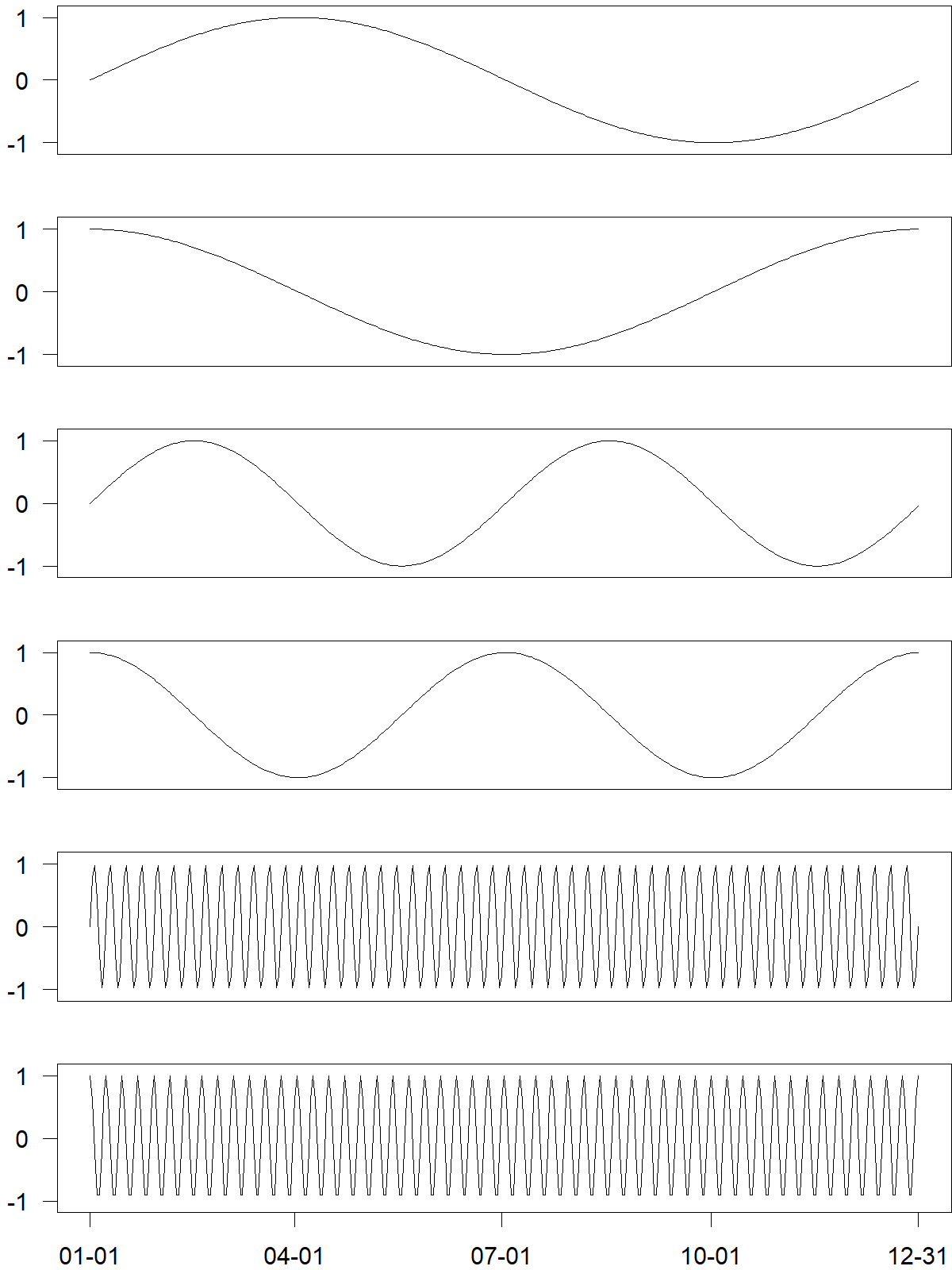
Figure 15.5: Predictors to model daily data with both intra-yearly (top four predictors) and intra-weekly (bottom two predictors) seasonality
For instance, we could transform dates using two sine and two cosine waves per year, to model intra-yearly seasonality, plus one sine and one coside wave per week, to model intra-weekly seasonality. In total, this would yield \(2\times 2+2\times 1=6\) predictors. Figure 15.5 shows the values of all six predictors over one year.
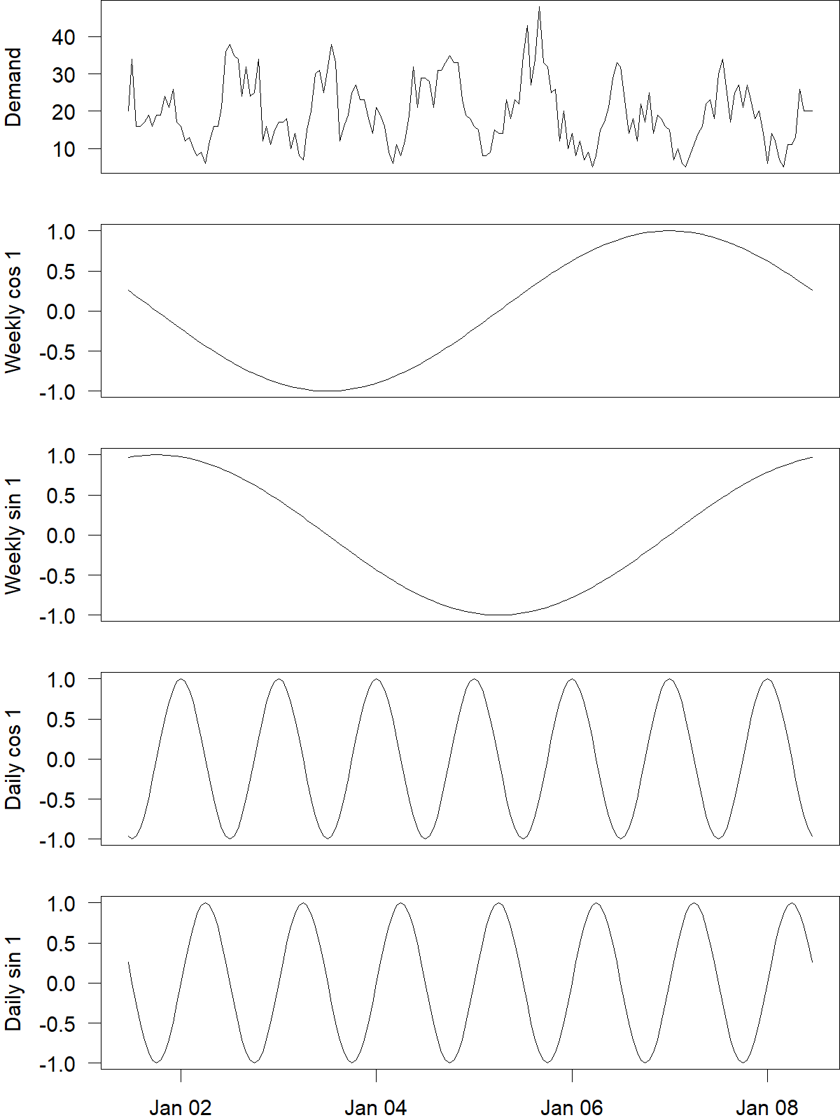
Figure 15.6: One week of hourly ambulance demand, with harmonics to model and forecast both intra-weekly and intra-daily seasonality
Figure 15.6 shows a sample of hourly ambulance demand at the top with harmonics we could use to model and forecast its multiple seasonalities below. Here, we use one harmonic with one sine and one cosine function each for the intra-weekly and the intra-daily seasonality. We could also use higher order sines and cosines to be more flexible as in Figure 15.5, always keeping in mind that flexibility will not automatically improve accuracy (see Section 11.7).
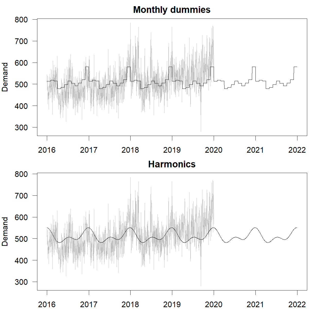
Figure 15.7: Daily ambulance demand with two different fits and forecasts modeling intra-yearly seasonality. Top: monthly dummies with questionable jumps between and constant values within months. Bottom: smoother forecasts based on two harmonics
Harmonics have two key advantages: we can model complicated seasonality with relatively few variables, and the behavior of these variables is smooth. To model the different hours in a week using harmonics, we would need much fewer terms than \(167\) dummy variables for the 168 hours a week (see below). To illustrate smoothness, consider the following example. Suppose we want to model monthly effects on daily data. We could use \(11\) dummy variables to model these effects, but using these variables in our model will imply that the forecast jumps rapidly from the last day of one month to the first day of the next – and then stays constant during the entire month, before suddenly jumping again at the beginning of the next month. Such patterns can be real (e.g., with regulatory or tax changes that take effect at the beginning of a month), but most seasonal effects occur more gradually. Figure 15.7 illustrates the difference between monthly dummy variables and harmonics for daily data with intra-yearly seasonality.
However, harmonics are less advantageous for modeling “regular” (i.e., short) seasonality. If we have daily data and want to model day-of-week patterns, then six dummy variables as illustrated in Table 15.2 work quite well. Similarly, we can use three quarterly dummy variables to forecast quarterly data or eleven dummy variables for monthly data.
15.6 Forecasting models for complicated seasonality
| Model | Predictors | Lagged Terms | Dummies | Harmonics |
|---|---|---|---|---|
| Simple average | Depends | Depends | Depends | Depends |
| MLR | Yes | Yes | Yes | Yes |
| MSARIMA | Yes | Auto | Yes | Yes |
| DSHW | No | No | Auto | No |
| TBATS | No | Auto | Yes | Auto |
| GAM | Yes | Yes | Yes | Yes |
| Prophet | Yes | Yes | Yes | Auto |
| MSTL | No | No | No | No |
| AI/ML | Yes | Yes | Yes | Yes |
Table 15.3 lists forecasting models and their capabilities to capture long, multiple or non-periodic seasonalities. Most forecasting models that are appropriate here use a mixture of lagged terms, seasonal dummies, and harmonics to deal with long and multiple seasonalities, or they can leverage predictors. In the following sections, we briefly review each forecasting model listed in Table 15.3. These models may vary in terms of accuracy, computational time, the ability of terms to evolve over time and flexibility. We refer to flexibility as the ability to incorporate different seasonal terms in the model. You may notice that in Table 15.3, Multiple Linear Regression (MLR) is a flexible model because it could use any of the dummy, harmonic, lagged terms or predictors; however, a model like Double Seasonal Holt-Winters (DSHW) is limited in terms of the types of seasonality that it can include, hence it is less flexible.
Simple averages of seasonal forecasts
A simple way to account for multiple seasonal patterns is to fit different seasonal forecasting models to the data and afterwards average the forecasts. As constituent models, we can use the ones we already know, like Exponential Smoothing or ARIMA for “simple” seasonality, or all the ones below for “more complicated” seasonality.
For example, suppose we have hourly data and suspect seasonal cycles within days, weeks, and years. Then we could fit three different seasonal forecasting models, with period lengths of \(m=24\) (24 hours in a day), \(m=168\) (168 hours in a week) and \(m=8766\) (8766 hours in a year), forecast each model out and take averages of the forecasts. The first model could be Exponential Smoothing or ARIMA, which can still deal with seasonality cycles of length 24, but for the longer weekly and yearly seasonalities, we would need to use one of the models below.
Multiple linear regression
Multiple Linear Regression (MLR) (see also Chapter 11) is a classic method to forecast time series with multiple seasonal cycles. For instance, you could create seasonal dummy variables to encode the day of the week, plus one or more harmonics to account for possible intra-daily and intra-yearly patterns, as in Figure 15.6. We can also model interactions between the different seasonal components if we have enough data.
MLR is a fast and flexible approach. It can allow for components to change over time by using weighted regression and weighting more recent observations more heavily. We can also decompose the contributions to seasonality stemming from the various model components (a process that becomes more challenging if we use interactions) for interpretation and debugging. In addition, MLR is available in most programming languages. We can also estimate MLR models quickly.
MLR is implemented in most statistical software packages, from base R to the scikit-learn (Pedregosa et al., 2011; scikit-learn core developers, 2023) and the statsmodels packages (Perktold et al., 2022) for Python.
Multiple/multiplicative seasonal ARIMA
The ARIMA model (see Chapter 10) has been extended to the Multiple/Multiplicative Seasonal ARIMA (MSARIMA) model to incorporate multiple seasonalities (J. W. Taylor, 2003). MSARIMA allows the inclusion of predictors, and the model components can evolve. However, the model is not very flexible, and the computational cost is very high.
More recently, Svetunkov and Boylan (2020) proposed Several Seasonalities or State Space ARIMA (SSARIMA). SSARIMA constructs ARIMA in a state-space form and allows modeling several seasonalities. While SSARIMA is flexible and allows for including predictors, its computational time to produce forecasts is also very high, especially for high-frequency time series.
R implements both MSARIMA and SSARIMA in the smooth package (Svetunkov, 2023).
Double seasonal Holt-Winters and variants
Researchers have extended the classical ETS methods (see Chapter 9). J. W. Taylor (2003) introduced a Double Seasonal Holt-Winters (DSHW) approach to model daily and weekly seasonal cycles, imposing the same intra-daily cycle for all days of the week. J. W. Taylor (2010) proposed a triple seasonal model, adding a separate seasonal state for the intra-daily, intra-weekly, and intra-yearly seasonalities to improve the model proposed by J. W. Taylor (2003). Gould et al. (2008) and J. W. Taylor and Snyder (2012) instead proposed an approach that combines a parsimonious representation of the seasonal states up to a weekly period.
While these models allow for evolving terms and decomposing components, their implementation is not flexible. Moreover, the models do not support the use of additional predictors. Their computational cost is also high.
R implements DSHW in the forecast package (Hyndman et al., 2023).
TBATS
An alternative approach to deal with long, multiple and non-periodic seasonalities is TBATS. This acronym stands for a method including (optional) trigonometric terms, Box-Cox transformations, ARMA errors, Trend and Seasonal components (De Livera et al., 2011). TBATS arranges these components in a completely automated manner. It also allows for terms to evolve.
Some drawbacks of TBATS, however, are that it is not flexible, can be slow to estimate and produce forecasts, and does not allow for predictors in the model. We refer interested readers to Section 12.1 of Hyndman and Athanasopoulos (2021) for more information.
R implements TBATS in the forecast package (Hyndman et al., 2023).
Generalized additive models and Prophet
Building on the foundation of the multiple linear regression methodology, Generalized Additive Models (GAMs) (Hastie and Tibshirani, 1990) allow non-linear relationships between the forecast variable and predictors. They can also include harmonics and any lagged terms or predictors in a way similar to MLR.
Facebook introduced Prophet (S. J. Taylor and Letham, 2018), which utilizes GAMs and accounts for strong seasonal effects through harmonics, piecewise trends, holiday effects (a dummy variable), and additional predictors. The implementation may be less flexible than MLR models, but it is robust to missing values, and structural changes in the trend and can handle outliers well. It is also an automated approach, which makes it easy to use.
The Prophet algorithm is implemented in the prophet package for Python (Facebook’s Core Data Science Team, 2022) and in the prophet package for R (S. Taylor and Letham, 2021).
Multiple seasonal-trend decomposition using loess
Alternatively, Bandara et al. (2021) propose an algorithm to decompose a time series into multiple additive seasonal components analogously to the standard STL decomposition for a single seasonal pattern (see Chapter 7). As in the standard STL decomposition, the different components can be forecasted separately and added together.
R implements the MSTL algorithm in the forecast package (Hyndman et al., 2023).
Artificial intelligence and machine learning
In parallel to the above developments, AI/ML methods are an alternative for forecasting time series with multiple seasonality. Neural networks, tree-based methods, Boosting, and other approaches described in Chapter 14 can include features for the hour of the day, the day of the week and the time of year (precisely as for multiple linear regression, see above) and model their effects. In principle, they can also detect and forecast interactions, like the effect of the hour of the day differing between different days of the week. However, as discussed in Section 14.5, AI/ML methods usually require much more data than adaptations of classical approaches.
Most AI/ML methods are implemented in various packages in Python, see e.g. Géron (2019), and many are also implemented in R.
Key takeaways
If seasonal cycles span many periods, traditional methods like Exponential Smoothing and ARIMA struggle.
Multiple seasonal patterns may overlap as we collect and store data on ever finer temporal granularities.
Cultural or religious events may have a regular impact that is not aligned with the standard Western calendar and may be non-periodic.
Whether multiple seasonalities have a significant impact can be analyzed using appropriate variations of seasonal plots.
One can use specialized methods or adapt standard causal models to address long, multiple, and complex seasonalities.