5 Know your time series
The first step in any analysis is to understand the data. In forecasting, this usually means understanding a time series – or many time series. In this chapter, we consider basic properties to look out for in your time series data, from data quality to the amount of data and its forecastability. We also consider the more technical issue of stationarity.
5.1 Data availability
A time series is a sequence of similar measurements taken at regular intervals. Examples of time series include the annual profits of Uber, quarterly unemployment rates in France, monthly donations to UNICEF, weekly sales at a retailer like Walmart, the daily Google stock price, or hourly hospital admission in the University Hospital of Wales. Every time series has two components: a time index, i.e., a variable that allows ordering observations from past to present, and a measurement, i.e., a numerical variable showing the observation corresponding to each time index.
Time series analysis, our topic in Chapters 8 to 16, means examining the history of the time series to obtain information about the future. An inherent assumption in time series analysis is that the past of a series contains information about the future of the same series. Causal models (Chapter 11) and Artificial Intelligence/Machine Learning algorithms (Chapter 14) use the information contained in another data series to predict the future of a focal time series.
One essential aspect of time series forecasting is that time needs to be bucketed into periods. Many demand forecasts are prepared monthly (“how much product will our customers demand next month?”), and thus, the time series requires aggregating data into monthly buckets. Note that a month is not an entirely regular time interval since some months have more days than others. Still, this non-regularity is inconsequential enough to be ignored for most applications. Some operational forecasting requires weekly, daily, and sometimes even quarter-hourly time buckets, for example, in the case of retail store-level forecasting (Fildes, Kolassa, et al., 2022; Fildes, Ma, et al., 2022) or call center traffic forecasting (Ibrahim et al., 2016). As we shall explain later in this chapter, this temporal dimension of aggregation implies different degrees of statistical aggregation, making forecasting more or less challenging. It also raises the question of temporal hierarchies (see Section 13.3). At what level should the organization forecast, and how does the organization aggregate or disaggregate to longer or shorter segments of time?
Another vital aspect to understand about our forecast is the availability of relevant historical data. Most methods discussed in the following chapters assume that some demand history for a time series exists. For example, suppose Exponential Smoothing is used (see Chapter 9), and the model includes seasonality. If our data are on quarterly granularity, we need at least nine past quarters’ observations to fit the model. And if we have monthly data, then we need a history of at least 17 months (Hyndman and Kostenko, 2007). These are minimum requirements; if the time series is very noisy, reliable parameter estimation requires much more data to be useful for forecasting. If too little data is available, the risk of detecting seasonality where none exists is much higher than the risk of failing to detect seasonality if it exists (see Section 11.7). So-called shrinkage or regularization methods are available to better deal with seasonality in such settings (Miller and Williams, 2003), or more generally, in situations with too little data.
This data requirement may be excessive in many business contexts, especially in industries with frequent introductions of new products. If product lifecycles are short, one must carefully assess the novelty of changes to the product portfolio. Do they represent new product introductions, that is, the introduction of a novel good or service incomparable to any existing product in the firm’s portfolio? Or do they represent a semi-new product introduction, a modified version of a product the firm has sold before (Tonetti, 2006)? In the former case, the methods we will discuss here do not hold; forecasts will require modeling the product lifecycle, which requires good market research and extensive conjoint analysis to have a chance of being successful (Berry, 2010). In the latter case, forecasting can proceed as we discuss here, as long as some existing data is representative of the semi-new product.
For example, suppose the semi-new product is a simple engineering change of a previous product version. In that case, the history of the earlier version of the product should contain information about the semi-new version. The earlier time series can thus initialize the forecasting method for the semi-new product. The time series level may change if the change is in packaging or style. Still, other components of the series, such as the trend, seasonality, and possibly even the uncertainty in demand, may remain constant. Thus, the estimates of these components from the past can be used for the new model as initial estimates, significantly reducing data needs.
Similarly, suppose the semi-new product is a new variant within an existing category. In that case, the current trend and seasonality estimates at the category level may apply to the new variant. In other words, intelligent top-down forecasting in a hierarchy (see Chapter 13) can allow forecasters to learn about these time series components by looking at the collection of similar variants within the same category.
The first step in time series analysis is understanding what data underlies the series. We frequently use sales rather than demand data as the input for demand forecasting. However, there is a difference between sales and demand, which comes into play during stockouts. If inventory runs out, customers may still demand a product so sales may be lower than the actual demand. In such a case, customers may turn to a competitor, delay their purchase, or buy a substitute product. In the latter case, the substitute’s sales are higher than its raw demand. Thus, demand forecasts based on historical sales data may be systematically wrong if this effect is significant and not taken into account. Modern forecasting software can adjust sales data accordingly if stockout information is recorded. The mathematics of such adjustments are beyond the scope of this book. We refer interested readers to Nahmias (1994) for further details.
Adjusting sales to estimate demand requires clearly understanding whether data represents sales or demand. Demand can be challenging to observe in business-to-consumer contexts. If a product is not on the shelf, it is hard to tell whether a customer walking through the store demands it. In online retail, we can observe demand if the website does not show inventory availability to the customers before they place an item into their shopping basket. However, if this information is presented to customers before they click on “purchase,” demand is again challenging to observe.
Demand is easier to observe in business-to-business settings since sellers usually record customer requests. In modern Enterprise Resource Planning (ERP) software, salespeople typically work with an available-to-promise number. Running out of available-to-promise means that the seller will not convert some customer requests into orders; if the salespeople do not record these requests, databases again only show sales, not demand.
5.2 How much data is necessary?
The amount of data we need to produce reliable forecasts depends on the context. As mentioned earlier, if your data has a trend or seasonality, we require more data history to estimate forecasting models successfully. In time series, the length of the time series should not be less than the number of parameters in the time series. For instance, the time series should have 24 months for a model to capture monthly seasonality (Chapter 6). Similarly, more history is needed to obtain reliable estimates if your data is noisy. How much data we need also depends on our forecast horizon. For example, forecasting 30 days out will require less data than forecasting 365 days out.
We may have a long time series, but consider throwing away old data, as it seems less useful. At what time does historical data become not worth the bother? Data processing may gradually take longer each day. Processes, products, and markets change over time, making older data apparently less relevant for current usage. Maybe you consider using a 5-year rolling period and discard the rest of your data. We would encourage you not to pursue this plan. In general, throwing away data is not a good practice. The more time series data you have, the better your model becomes. Having more data is especially important if you represent the forecast as a probability density distribution where the distribution’s tails provide crucial information to deal with risk. Having a longer history makes your time series more representative – it will include all the ups and downs that your market has experienced and may yet experience again. More time series data means more information about the past.
Also, many forecasting models, such as Exponential Smoothing, can handle the underlying process, product, or market changes. If you use such a model, there are no issues with using a long history of a time series as an input to the model because the model will recognize and adjust to those changes. If you throw away old data, you risk not being able to capture longer-term trends. You may also fail to get reasonable estimates for special events like Christmas. Lastly, your model may under-estimate the uncertainty in your time series.
Another dimension to consider is the number of predictors (see Chapter 11) you use in your model. While using longer historical time series is usually useful, using more predictors is not necessarily beneficial. Spurious relationships may appear, and valuable information becomes less apparent (see Section 11.7). It would be best to have a handful of quality predictors that can describe the underlying variation rather than a grab bag of predictors with lower predictive quality.
5.3 Data quality
Good quality data is indispensable for any data science task. This truism holds in a time series forecasting context. There are many ways in which data can be wrong, corrupted, “bad,” or simply inexistent. How critical it is to have quality data will depend on what time series process you are modeling. How to detect and address data quality issues depends on the context. Here are a few examples:
Figure 4.5 shows daily sales of a specific SKU in a particular store. We notice a period of zero sales about one-third of the way through the series. Given that this product is otherwise relatively fast selling, we suspect that these zero sales were not caused by sudden low demand but by a stockout. The data are censored. The problem may be minor in this case. But other products may have longer stockouts, and these may have an impact on the forecasting model. Imagine an out-of-stock around Christmas – will our forecast for next year’s Christmas be zero because the system thought that demand decreased systematically in this time?
If some sensor or process collects our time series, we may not have any data for some periods because the sensor or process broke down. Our data preparation pipeline should catch and alert us to such problems. If we forget sanity checking, we could feed missing data as zero observations into our forecasting model.
Retailers generally record their historical sales but sometimes fail to register their historical promotions. Without knowing when promotions occurred in the past, it is tough to forecast the impact of future promotions.
Data may be corrupted, especially if any processing steps are involved. If we pull our time series out of a database via manual selection, joining, and aggregation steps, it is easy for errors to creep in and remain undetected.
One frequently overlooked aspect of data quality is accuracy measurement. If we assess our forecast accuracy using a holdout sample, and the data in that holdout period is problematic, we may draw completely wrong conclusions. Imagine that we had a stockout and censored retail data during the holdout period – any forecast close to zero would look very good, despite actual unconstrained demand being likely much higher. Optimizing our forecasts against bad-quality data can thus lead to systematically biased predictions. Evaluating forecasts against stockout periods is an excellent recipe to produce forecasting models that predict zero demand – i.e., models that drive us out of business.
How do we systematically detect such data quality issues? As there are so many different ways in which data quality can deteriorate, we can only provide a few general hints here.
It is always a good idea to plot a time series – ideally on multiple levels of aggregation because sometimes data quality problems only become apparent in the aggregate (just as they are sometimes only visible at a finer granularity). Plot several series, get a cup of coffee, and flip through the series. If anything looks wrong, consider whether it is and what may cause it. And do the same for any holdout data you may have to ensure you are not training and evaluating your forecasting models on bad data. It is always enlightening to look particularly at those time series that a method forecasts exceptionally well or poorly. A single outlier due to a data entry error can significantly impact forecast accuracy. Therefore, such an error can also be easily found and corrected by filtering time series for bad forecasts (which may actually be good ones and only look bad because we evaluate them against problematic data).
Once we have identified data quality issues, what can we do about them? Again, this depends on the domain in which we are and the forecasting method. If we have found a problem with our data preparation step, we might be able to correct the preparation and re-run it, ending up with correct and clean data. However, there is not always such a happy ending to our data cleansing efforts. What do we do with problematic data when we can’t pull the correct and clean data from somewhere?
Some methods, like regression models (see Chapter 11) or tree-based methods (see Section 14.2), have no problem with missing data, so we can simply remove the problematic data points. Other methods, like ARIMA (see Chapter 10) or Exponential Smoothing (see Chapter 9), have significant issues with missing data, so we can’t just remove problematic data points. We must replace them. Unfortunately, what to replace such problematic data with can be a science all its own. We could take the average of the last valid data point before the problem and the first sound data point after the problem. However, if we have a long string of problems (e.g., if our sensor was out for a more extended period), that will give us a long period of imputed constant values, which can dominate our forecasting model. Alternatively, we can fit some model to the valid data and predict the problematic periods. In this case, we are back to square one: to replace our problematic data to fit a forecasting model, we must choose a good “data replacement model.” But to decide whether such a model is “good,” we need to rely on the sound data we do have.
All this can get complicated, and there is an art to knowing how much time and effort to invest in cleaning data (and searching for data problems in the first place) and subsequently modeling the cleaned data. The key is to remember that data cleansing is always necessary. It always takes longer than anticipated, but it can yield significant benefits. Often, cleaning the input data leads to more substantial forecast improvements than trying more complicated algorithms on less clean data.
5.4 Stationarity
One key attribute of a time series is stationarity. Stationarity indicates that the mean of demand is constant over time, that the variance of demand remains constant, and that the correlation between current and most recent demand observations (and other parameters of the demand distribution) remains constant. Stationarity, in essence, requires that the time series has stable properties when looked at over time.
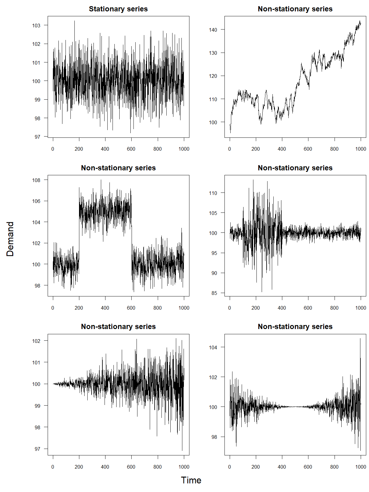
Figure 5.1: Examples of a stationary versus non-stationary time series
Many time series violate these criteria; for example, a time series with a trend (see Chapter 7) is not stationary since the mean demand is persistently increasing or decreasing. Similarly, a simple random walk (see Chapter 7 and Section 8.2) is not stationary since mean demand randomly increases or decreases in every period. In essence, non-stationary series imply that demand conditions for a product change over time, whereas stationary series imply that demand conditions are very stable. Some forecasting methods work well only if the underlying time series is stationary. Others, such as the ARIMA methods discussed in Chapter 10, preprocess the data (in the case of ARIMA models, by differencing; see Section 10.2) in an attempt to make it stationary. Figure 5.1 provides a few examples to illustrate the difference between stationary and non-stationary time series.
We often transform time series to become stationary before they are analyzed. Typical data transformations include first differencing, that is, examining only the changes of demand between periods; calculating growth rates, that is, examining the normalized first difference; or taking the natural logarithm of the data. Suppose, for example, one observes the following four observations of a time series: 100, 120, 160, and 150. The corresponding three observations of the first difference series become 20, 40, and –10. Expressed as growth rates, this series of first differences becomes 20, 33, and –6%.
These transformations are reversible. While we make estimations on the transformed data, we can transform the resulting forecasts back to be useful for our purpose. The benefit of such transformations usually lies in the reduction of variability and in filtering out the unstable portions of the data. Statistical software generally reports several statistical tests for stationarity, such as the Dickey–Fuller test. Applying these tests to examine whether a first-differenced time series has achieved stationarity is helpful.
5.5 Forecastability and scale
Another aspect to understand about a time series is the forecastability of the series. As discussed in Chapter 1, some time series contain more noise than others, making predicting their future realizations more challenging. The less forecastable a time series is, the wider the prediction interval associated with the forecast will be. Understanding the forecastability of a series not only helps set expectations among decision-makers but is also essential when examining appropriate benchmarks for forecasting performance. Competitors’ forecasts may be more accurate if they have a better forecasting process, or if their time series are more forecastable. The latter may simply be a result of them operating at a larger scale, with less variety, or their products being less influenced by current fashion and changing consumer trends.
One measure of the forecastability of a time series is the ratio of the standard deviation of the time series to the standard deviation of errors for forecasts calculated using a benchmark method as per Chapter 8 (Hill et al., 2015). The logic behind this ratio is that the standard deviation of demand is, in some sense, a lower bound on performance since it generally corresponds to using a simple, long-run average as your forecasting method for the future. Any proper forecasting method should not lead to more uncertainty than the uncertainty inherent in demand. Thus, if this ratio is \(>1\), forecasting a time series may benefit from more complex methods than a long-run average. If this ratio is close to 1 (or even \(<1\)), we may not be able to forecast the time series any better than using a long-run average.
This conceptualization resembles what some researchers call Forecast Value Added (Gilliland, 2013). In this concept, one defines a base accuracy for a time series by calculating the forecast accuracy achieved (see Chapter 17) by the best simple method (see Chapter 8). Every step in the forecasting process, whether it is the output of a statistical forecasting model, the consensus forecast from a group, or the judgmental adjustment to a forecast by a higher-level executive, is then benchmarked in terms of their long-run error against this base accuracy. If a method requires effort from the organization but does not lead to better forecast accuracy compared to a method that requires less effort, we can safely eliminate it from future forecasting processes. Results from such comparisons are often sobering. Some estimates suggest that in almost 50% of time series, the existing toolset available for forecasting does not improve upon simple forecasting methods (Morlidge, 2014a). In other words, demand averaging or simple demand chasing may sometimes be the best a forecaster can do to create predictions.
Some studies examine what drives the forecastability of a series (Schubert, 2012). Key factors include the overall volume of sales (larger volume means more aggregation of demand, thus less observed noise), the coefficient of variation of the series (more variability relative to mean demand), and the intermittency of data (data with only a few customers who place large orders is more difficult to predict than data with many customers who place small orders). In a nutshell, we can explain the forecastability of a time series by product characteristics as well as firm characteristics within its industry. There are economies of scale in forecasting, with forecasting at higher volumes being easier than forecasting for low volumes.
The source of these economies of scale lies in the principle of statistical aggregation. Imagine trying to forecast who among all the people living in your street will buy a sweater this week. You would end up with a forecast for each person living in the street that is highly uncertain for each individual. However, the task becomes much easier if you just want to forecast how many people living in your street buy a sweater in total. You can make many errors at the individual level, but at the aggregate level, these errors cancel out. This effect will increase the more you aggregate, predicting at the neighborhood, city, county, state, region, or country level. Thus, the forecastability of a series is often a question of what level of aggregation a time series focuses at. Very disaggregate series can become intermittent and, therefore, very challenging to forecast (see Chapter 12 for details). Very aggregate series are easier to forecast, but if the level of aggregation is too high, these forecasts become less useful for planning purposes, as the information they contain is not detailed enough.
It is vital in this context to highlight the difference between relative and absolute comparisons in forecast accuracy. In absolute terms, a series at a higher level of aggregation will have more uncertainty than each individual series. Still, in relative terms, the uncertainty at the aggregate level will be less than the sum of the uncertainties at the lower level. Suppose you predict whether a person will buy a sweater or not. In that case, your absolute error is at most 1, whereas the maximum error of predicting how many people in your street buy a sweater or not depends on how many people live in your street; nevertheless, the sum of the errors you make at the individual level will be less than the error you make in the sum. For example, suppose five people live in your street, and we can order them by how far they live in the street (i.e., first house, second house, etc.). You predict that the first two residents will buy a sweater, whereas the last three do not. Your aggregate prediction is just that two residents buy a sweater. Suppose now that only the last two residents buy a sweater. Your forecast is 100% accurate at the aggregate level but only 20% accurate at the disaggregate level. Generally, the standard deviation of forecast errors at the aggregate level will be less than the sum of the standard deviations of forecast errors made at the disaggregate level.
Supply chain design can allow using more aggregate forecasts in planning. The benefits of aggregation here are not limited to better forecasting performance but also include reduced inventory costs. For example, the concept of postponement in supply chain design favors postponing the differentiation of products until later in the process. This practice enables forecasting and planning at higher levels of aggregation for longer within the supply chain. Paint companies were early adopters of this idea by producing generic colors that are mixed into the final product at the retail level. This postponement of differentiation allows forecasting (and stocking) at much higher levels of aggregation. Similarly, Hewlett-Packard demonstrated how to use distribution centers to localize their products. This allowed them to produce and ship generic printers to distribution centers.
A product design strategy that aims for better aggregation is component commonality or a so-called platform strategy. Here, components across stock-keeping units are kept in common, enabling production and procurement to operate with forecasts and plans at a higher level of aggregation. Volkswagen is famous for pushing the boundaries of this approach with its MQB platform, which allows component sharing and final assembly on the same line across such diverse cars as the Audi A3 and the Volkswagen Touran. Additive manufacturing may become a technology that allows planning at very aggregate levels (e.g., printing raw materials and flexible printing capacity), allowing companies to deliver various products without losing economies of scale in forecasting and inventory planning.
5.6 Using summary statistics to understand your data
Using summary statistics, such as the mean (average) and the standard deviation is an initial step to understand data, as discussed above. These measures may help to condense data, compare different datasets, and convey complex messages.
While summary statistics can provide a basic understanding of data, however, their usefulness for time series analysis is limited. First, they cannot highlight patterns in the data, identify unusual observations, describe changes over time, or help to understand relationships between variables. Second, they could be misleading. For example, a set of four datasets known as Anscombe’s Quartet, as well as another collection of 13 datasets called the Datasaurus Dozen, each have the same summary statistics – means and standard deviations of both variables, as well as correlations – but are completely different when plotted (Matejka and Fitzmaurice, 2017). Thus, similar statistics can stem from very different datasets. Therefore, we should never rely exclusively on summary statistics alone in our judgment and always visualize our data.
Visualising data can communicate information much quicker than summary statistics and provides a better tool for analyzing and understanding time series data. In Chapter 6 we will see how different time series graphics can be used to better understand data.
Key takeaways
Understanding your data is the first step to a good forecast.
The objective of most forecasts is to predict demand, yet the data available to prepare these forecasts often reflects sales; if stockouts occur, sales are less than demand.
Many forecasting methods require time series to be stationary, that is, to have constant parameters over time. We can often obtain stationarity by suitable transformations of the original time series, such as differencing the series.
A vital attribute of a time series is its forecastability. Your competitors may have more accurate forecasts because their forecasting process is better or their time series are more forecastable.
There are economies of scale in forecasting; predicting at a larger scale tends to be easier due to statistical aggregation effects.
Throwing away time series data just because it is “old” is not a good practice. The longer your time series, the better your model becomes.
Do not rely on summary statistics alone to understand your data; always plot your data.