12 Count data and intermittent demand
The forecasting methods we have introduced so far implicitly assumed continuous demand and used the normal distribution (see Figure 3.1) “under the hood.” This is a reasonable approximation for fast moving products. In this chapter, we discuss specialized forecasting methods that are better suited to dealing with slow moving products.
12.1 Definitions
So far, we have focused on using the normal distribution for forecasting. Using the normal distribution can be inappropriate for two reasons: First, the normal distribution is continuous, i.e., a normally distributed random variable can take non-integer values, like 2.43. Second, the normal distribution is unbounded, i.e., a normally distributed random variable can take negative and positive values. Both these properties of the normal distribution do not make sense for (most) demand time series. Demand is usually integer-valued, apart from products sold by weight or volume, and demand is usually zero or positive, but not negative, apart from returns.
These seem obvious ways in which the normal distribution deviates from reality. So why do we nevertheless use this distribution? The answer is simple and pragmatic: because it works. On the one hand, using the normal distribution makes the statistical calculations that go on “under the hood” of your statistical software (optimizing smoothing parameters, estimating ARIMA coefficients, calculating prediction distributions, etc.) much more manageable from a mathematical point of view. On the other hand, the actual difference between the forecasts – point, interval and distribution – under a normal or a more appropriate distribution is often tiny, especially for fast-moving products. However, this volume argument supporting the normal distribution does not hold for slow-moving demand time series.
We can address both above-mentioned problems by using count data distributions, i.e., random number distributions that only yield integer values. Common distributions to model demands are the Poisson and the negative binomial distribution (Boylan and Syntetos, 2021; Syntetos et al., 2011). The Poisson distribution has a single parameter representing its mean and variance. The more flexible negative binomial distribution has one parameter for the mean and another one for its variance or its over-dispersion (i.e., the amount by which the variance of the distribution exceeds its mean).
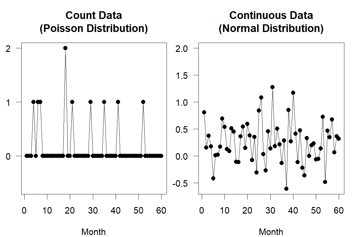
Figure 12.1: Random draws for count data and continuous data for low-volume products with mean and variance both equal to 0.2. The right-hand panel obviously cannot correspond to demand of a real product
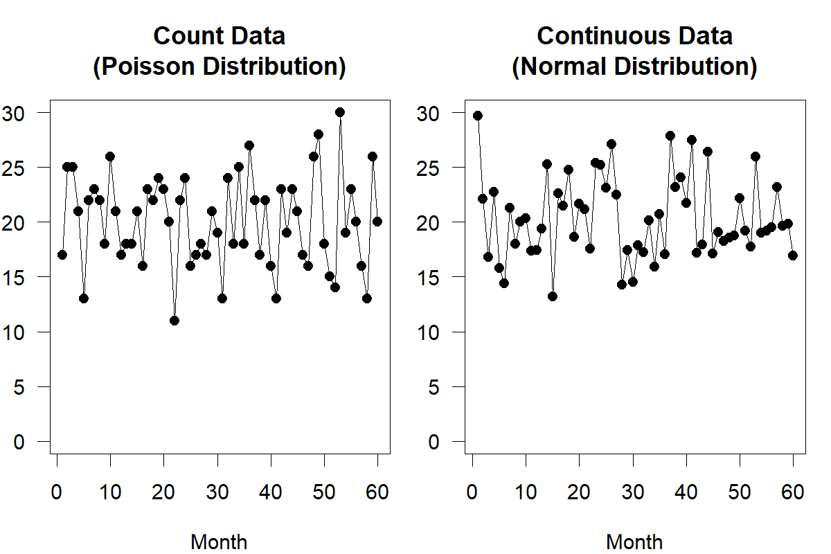
Figure 12.2: Random draws for count data and continuous data for high-volume products with mean and variance both equal to 20
Figure 12.1 illustrates the difference between Poisson-distributed and normally distributed demand at a rate of 0.2 units per month. We see both problems discussed above (negative and non-integer demands) in the normally distributed data, whereas the Poisson time series does not exhibit such issues and therefore appears more realistic. Conversely, Figure 12.2 shows little difference between a Poisson and a normal distribution for fast-moving products – here, at a rate of 20 units per month. Thus, we can reasonably model fast moving products (as in Figure 12.2) using a normal distribution, but not slow moving products (as in Figure 12.1).
Once demand gets so slow that buckets exhibit zero demand many times, we speak of intermittent demand series. We will interchangeably use the terms count data and intermittent demand.
Finally, there is lumpy demand. Demand is “lumpy” if it is intermittent and non-zero demands are high. Lumpy demand can occur, for instance, for upstream supply chain members with only a few customers that place batch orders. Another example is home improvement retail or wholesale stores, where builders typically buy large quantities of a particular paving stone or light switch at once. Low-volume intermittent data often results from many customers placing orders rarely; high-volume lumpy demand results from a few customers aggregating their orders into large batches. We illustrate the differences and similarities between these concepts in Figure 12.3.
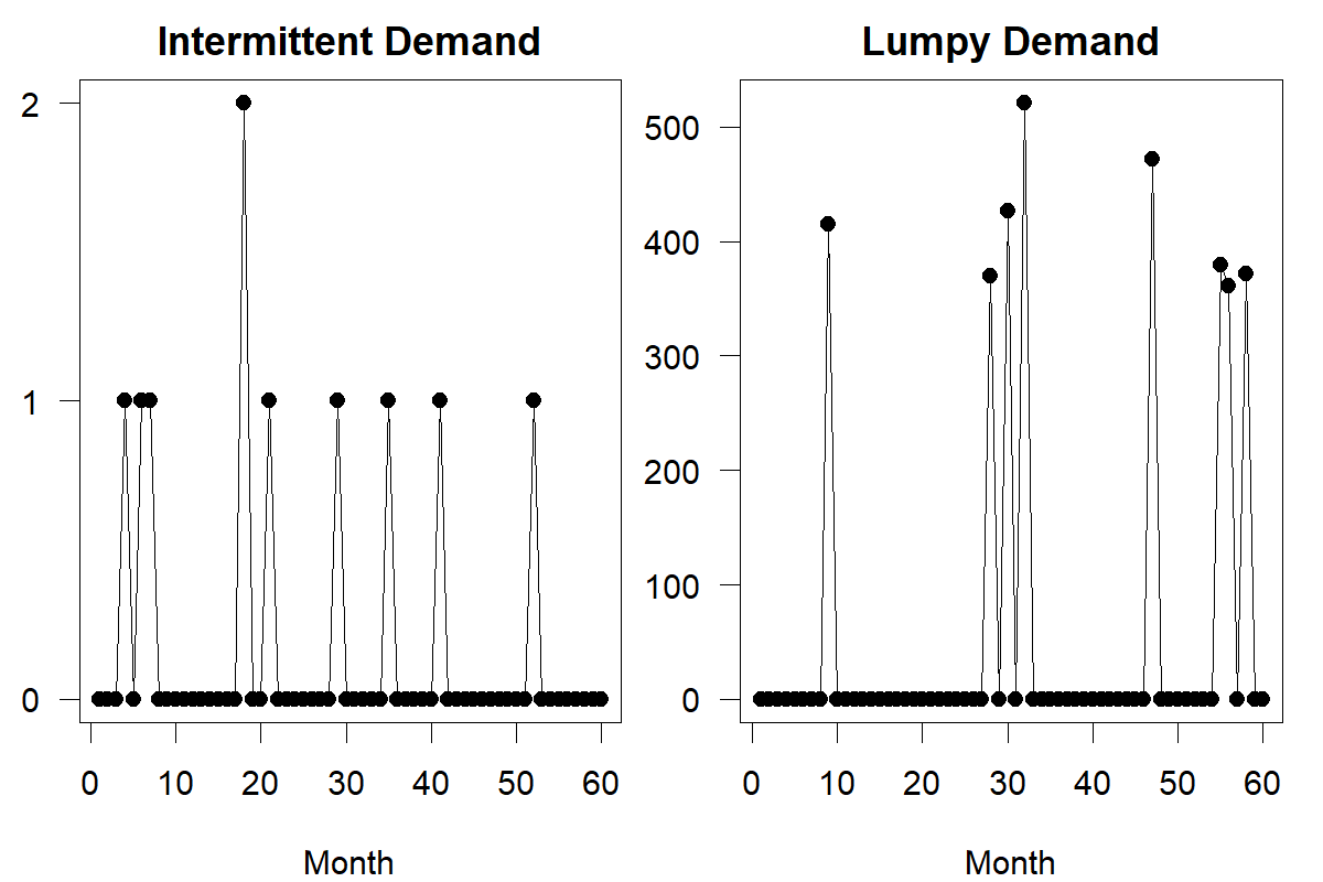
Figure 12.3: Intermittent and lumpy demand series. Note vertical axes.
Why is it important to forecast intermittent or lumpy demand? We naturally focus on forecasting the fastest-moving products simply because these products have the highest visibility in the firm (and market) and are often the most important in terms of margin and total revenue. However, most businesses also have a Long Tail of slow-moving products. By the anecdotal Pareto principle, 80% of your SKUs will be responsible for 20% of your sales. Classic A-B-C analysis in inventory management naturally differentiates between these fast- and slow-moving items. Many of these 80% of SKUs probably have intermittent demand series. While improving the forecasts for the 20% of fast-movers that drive 80% of sales is crucial, the many more slow-movers may represent a much more significant fraction of your total inventory value. Accurate forecasts can help you reduce these inventories, pool them, move to a make-to-order process, or generally improve your operations. There may be as significant an improvement opportunity here as there is for faster-moving items.
In addition, intermittent time series occur more and more frequently due to several recent developments. In the past, database capacity and processing power limited the number of demand time series to be stored and forecasted weekly. Nowadays, vastly more powerful storage and processing (Januschowski et al., 2013) allow working with ever-lower granularity. And a time series that is fast-moving on a weekly basis may well be slow-moving on a daily basis and can be heavily intermittent on an hourly basis. The more we disaggregate the time unit used for forecasting, the more likely we are to encounter intermittent data.
Further, a small product portfolio that slices a market into only a few segments by only providing a small number of product variants will likely produce high-volume series. However, with more and more product differentiation, many variants may become intermittent in demand. Thus, due to increased product variety and data storage capacity available, we need to forecast more and more intermittent time series.
12.2 Traditional forecasting methods
Given the particularities of intermittent demand, how should we forecast series with such count data? Could we also use the methods described in the previous chapters in this context?
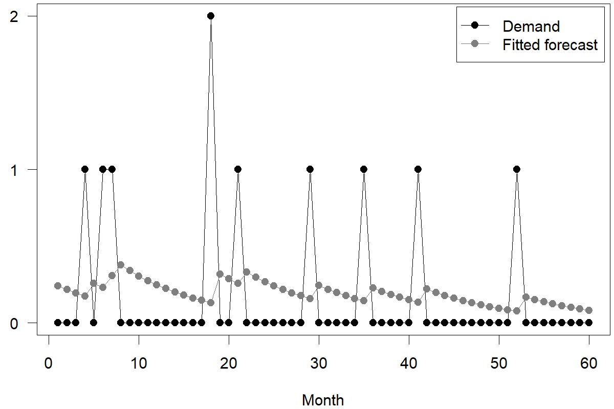
Figure 12.4: Single Exponential Smoothing applied to an intermittent time series
Let us apply Single Exponential Smoothing (see Chapter 9) with a smoothing parameter of \(\alpha = 0.10\) to an intermittent demand series in Figure 12.4. Remember that Single Exponential Smoothing creates forecasts by calculating a weighted average between the most recent forecast and the most recent demand. Thus, the forecasts tend to slowly move toward zero when we observe no demand. After we observe some demand, forecasts briefly jump up again. Thus, our forecast is high after a non-zero demand and low after a long string of zero demands.
This form of forecasting does not make sense in two critical situations. First, consider a context where our intermittent demand is driven by a few customers who replenish this SKU when needed. In this case, we would need a higher forecast (and not a lower forecast) after a long string of zero demands because it becomes more likely that these customers will place an order again as more time passes. Second, suppose we have a context where the intermittent demand is driven by many customers buying independently (but rarely). In that case, the forecast should not exhibit any time dynamics because, at any point in time, an equally large pool of customers may soon demand the product, even after one particular customer has just bought it.
Another problem with applying Exponential Smoothing to intermittent demands is that we typically make replenishment or production decisions right after a sale depletes our stock. So forecasts that are biased high right after sales will lead to particularly high reorder quantities and unnecessarily high inventories. To overcome these problems, we will now focus on a method to overcome these challenges.
12.3 Croston’s method
Croston (1972) examines the problem of forecasting intermittent demand and proposes a specific solution to this problem. This solution is by now an industry standard and bears Croston’s name. Instead of Exponentially Smoothing the raw demands, we separately smooth two different time series:
- all the non-zero demands from the original time series and
- the number of periods with zero demands between each instance of non-zero demand.
In a sense, we decompose the forecasting problem into the sub-problems of predicting how frequently demand happens and predicting how high the demand is if it happens. We highlight the values associated with these two time series in Figure 12.5.
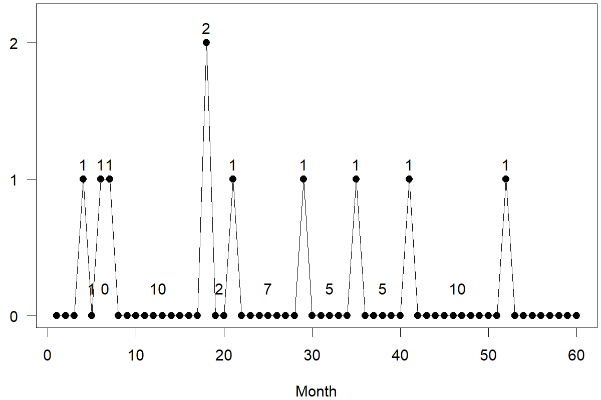
Figure 12.5: Demand and time periods without demand in an intermittent series
Thus, the problem becomes one of separately forecasting the series of non-zero demands, that is, (1, 1, 1, 2, 1, 1, 1, 1, 1), and the series of periods that are zero in-between demands, that is, (1, 0, 10, 2, 7, 5, 5, 10) in Figure 12.5. Croston’s method applies Exponential Smoothing to both these series separately (usually with the same smoothing parameters). Further, we only update the two Exponential Smoothing models and forecasts for these two series whenever we observe a non-zero demand.
Let us assume that smoothing the non-zero demands yields a forecast of \(q\), while smoothing the numbers of zero demand periods yields a \(r\). This means that we forecast non-zero demands to be \(q\), while we expect such a non-zero demand once every \(r\) periods on average. Then, the demand point forecast in each period is simply the ratio between these two forecasts, that is,
\[\begin{align} \mathit{Forecast} = q / r \tag{12.1} \end{align}\]
Croston’s method works through averages; while it is not designed to predict when a particular demand spike occurs, it essentially distributes the volume of the predicted subsequent demand spikes over the expected periods until that demand spike occurs. One could also think of Croston’s method as predicting the ordering behavior of a single client with fixed ordering costs. According to the classic Economic Order Quantity model, a downstream supply chain partner will lump continuous demand into order batches to balance the fixed cost of order/shipping with the variable cost of holding inventory. According to that logic, we could view Croston’s method as a way of predicting the demand this downstream supply chain partner sees – that is, to remove the order variability amplification caused by batch ordering from the time series. Figure 12.6 provides an example of how Croston’s method fits and forecasts an intermittent demand series.
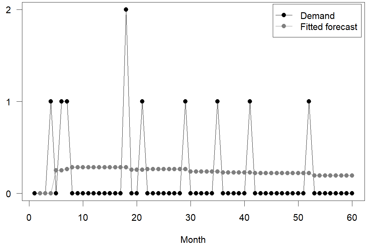
Figure 12.6: Croston’s method applied to an intermittent demand time series
Croston’s method provides some temporal stability of forecasts. Still, it does not address the problem that, for a small number of customers, long periods of non-ordering should indicate a higher likelihood of them placing an order. Further, Croston’s method works by averaging and forecasting the rate at which demand comes in, not by predicting when demand spikes occur; this makes it hard to interpret forecasts resulting from Croston’s method for decision-making. The forecast may say that on average over the next five weeks, we will sell one unit each week – where there is likely only one week during which we sell five units.
A closer theoretical inspection shows that Croston’s method suffers from a statistical bias (Syntetos and Boylan, 2001). Technically, this bias occurs because Equation (12.1) involves taking expectations of random variables, and because the expectation of a ratio is not equal to the ratio of the separate expectations. Modern forecasting software has proposed and implemented various correction factors to compensate for this problem. One example of such a correction procedure is the Syntetos–Boylan approximation (Syntetos and Boylan, 2005; Teunter and Sani, 2009), which has often led to better inventory positions (Syntetos et al., 2015).
Croston’s method is straightforward and may appear “too simple.” Why is it nevertheless very often used in practice? One factor is its simplicity (compare Chapter 8) – we can explain it quickly, and the logic underlying the method is intuitive to understand. Another explanation may be that intermittent demand often does not exhibit many dynamics that can be modeled. It is tough to detect seasonality, trends, or similar effects in intermittent demands, so trying to create a more complex model quickly runs into overfitting issues (see Section 11.7). The literature nevertheless proposes several competing models for intermittent demands. Still, their added complexity needs to be weighed against any gain in accuracy compared to Croston’s method – and no other method has so far consistently outperformed Croston’s method with the Syntetos–Boylan approximation.
That said, there is one situation in intermittent demand forecasting where Croston’s method performs poorly, namely, for lumpy demands. Suppose we have a demand of one unit once every 10 weeks (non-lumpy demand) or ten units once every 100 weeks (lumpy demand). In both cases, the average demand is 1/10 = 10/100 = 0.1 unit per week. Croston’s method will yield forecasts of about this magnitude in both cases. However, the two cases have very different implications for inventory holding. Failing to differentiate between these two situations is not a shortcoming of Croston’s method per se because a point forecast of 0.1 is an entirely accurate summary of the long-run average demand. The problem is that the point forecast does not consider the spread around the average.
Unfortunately, there is no commonly accepted method for forecasting lumpy demands for inventory control purposes. Most forecasters use an ad hoc method like “stock up to the highest historical demand” or a standard forecasting method with high safety stocks. They may also try to reduce their reliance on forecasting for such time series by managing demand and moving to a make-to-order system as much as possible. The challenges of intermittent demand forecasting are one reason why spare parts inventory systems (generally with intermittent demand patterns) increasingly utilize additive manufacturing to print spare parts on demand (D’Aveni, 2015).
Standard forecast accuracy metrics can exhibit very surprising behavior when applied to intermittent or lumpy time series. For instance, the MAE will very often be smallest for a flat zero forecast. Thus, paying attention to error metrics is even more important in intermittent or lumpy contexts. See Section 17.4 for details.
Croston’s method is implemented in the forecast (Hyndman et al., 2023) and fable (O’Hara-Wild et al., 2020) packages for R and in the croston package for Python (Mohammadi, 2022).
Key takeaways
Count data and intermittent demands are probably responsible for only 20% of your sales but may account for 80% of your inventory costs. Therefore, it makes sense to invest in forecasting them well.
Do not use Exponential Smoothing or ARIMA to forecast intermittent demands. Instead, use Croston’s or other methods dedicated to intermittent series. Pay particular attention to the connections between forecasts and inventory control.
If you can expand the time unit or aggregate across locations, you can often convert intermittent time series into non-intermittent series that are easier to forecast.
Lumpy demands are challenging to forecast since the average rate may be useless for inventory control.
Forecast accuracy metrics can be very misleading in intermittent or lumpy contexts. Be careful!