13 Forecasting hierarchies
Forecasts inform many organizational decisions, on inventories, capacity, staffing, cash flow, and budgets. These decisions happen at different organizational levels (e.g., firm vs. division vs. unit) and in different time granularities (e.g., daily, monthly, quarterly, or yearly). Accordingly, time series have natural hierarchical structures in “structural” and temporal dimensions (Seaman and Bowman, 2022; Syntetos et al., 2016). If we simply forecast each hierarchy level separately, then the forecasts will typically not be coherent: the sum of lower level forecasts will not be equal to the higher level forecast, although historical sales are of course coherent. In addition, lower-level time series are detailed but noisy, whereas higher level series are less noisy but can lack detail. The present chapter addresses forecasting in hierarchies and discusses various ways of achieving coherence (and also discusses when coherence is not called for).
13.1 Structural hierarchies
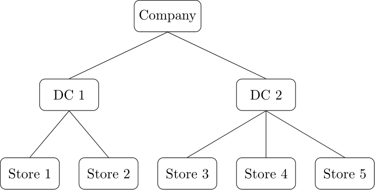
Figure 13.1: A simple location hierarchy for a company with two distribution centers (DCs) serving five stores
The first kind of hierarchy that comes to mind is the structural kind, which comes in three main variants: (a) organizational, (b) location or geographical and (c) product hierarchies. In the organizational dimension, a company is typically divided into different divisions that address different market segments. In the location hierarchy, we may have groupings of activities by country or region, or our supply chain may be regionally organized. Figure 13.1 gives a simple example of a location hierarchy. Finally, in the product dimension, products are usually organized in a product hierarchy that groups Stock Keeping Units (SKUs) into products or product groups, these into brands, and these again possibly into categories – where the precise categorization differs very much by industry.
Bills of materials also create hierarchical structures among our products: Suppose we bake both blueberry and chocolate chip muffins. We need forecasts for the demands for both muffin types separately to plan production, but when sourcing flour, we only need a forecast of our total flour demand. We do not care which kind of muffin we use a particular pound of flour for. The historical consumption of flour equals the sum of the consumptions for the two different muffin types. But if we separately forecast flour demand for each muffin type and total flour demand, the two lower level forecasts will not add up to the higher level one.
Product proliferation and the creation of more and more product variants tends to increase the complexity of the product hierarchy, and market differentiation may have similar effects on organizational or location hierarchies.
Structural hierarchies may be nested or crossed. An example of a nested hierarchy would be if the product hierarchy is nested within the organizational hierarchy of the company – or in other words, the company is organized by product considerations. However, if all products are sold in different geographies, then the location and the product hierarchy are crossed. In a business-to-business context, we also often deal with specific customers or accounts, which will likely go across products, possibly even across our geographical and organizational hierarchy.
We come across challenges when the manufacturing division requires a forecast per SKU across all geographies. While an account manager needs a forecast of demand from their main accounts within a geography but across all products, a marketing manager asks for a forecast of total demand for a single brand within a geography, across all products in that brand. A brand manager at a Consumer Packaged Goods company plans marketing campaigns that affect all SKUs in a brand; a distribution center (DC) needs to plan capacity and staffing to support the stocking and movement of all SKUs assigned to the DC. Demand planners work with product-level demand data, but financial planners report revenues at the division or company level. A retail company may need store-specific forecasts for particular SKUs to determine the store replenishment policy, but it will also need forecasts for the same SKUs at its DC, which serves many stores, to plan the replenishment of the DC. In business-to-business settings, salespeople may need customer-specific forecasts, whereas production planners need a forecast of the total demand across all customers. A consumer goods manufacturer may be interested in sales of a specific SKU to retailer A in region X and to retailer B in region Y, crossing the geographical and customer hierarchies.
Of course, we could always pull the historical data appropriate for each forecast and fit a model to this data. However, if we calculate all such forecasts separately, they will be almost completely independent and will not be guaranteed to be coherent, and we will not be leveraging “similar” slices through the data cube in any way. We will consider different methods of addressing these issues in the next section.
13.2 Forecasting hierarchical time series
Suppose we ignore the hierarchical and interdependent nature of our forecasting portfolio. In that case, we could take the time series at the different aggregation levels – say, sales of SKU A, B and C, and total sales in the category containing A to C – as independent time series and forecast them separately. The problem with this approach is that the forecasts will not be coherent. Whereas the historical demands of the different SKUs add up to the total historical category demand, the forecasts of the different SKUs will almost certainly not add up to the forecast on the category level. “The sum of the forecasts is not equal to the forecast of the sum.”
There are various ways of addressing this problem, all with advantages and disadvantages, which we will describe next. Figure 13.2 shows a simple example product hierarchy consisting of three SKUs, each with three years of simulated history and one holdout year. In the following sections, we will work with this hierarchy and show coherent forecasts derived in different ways.
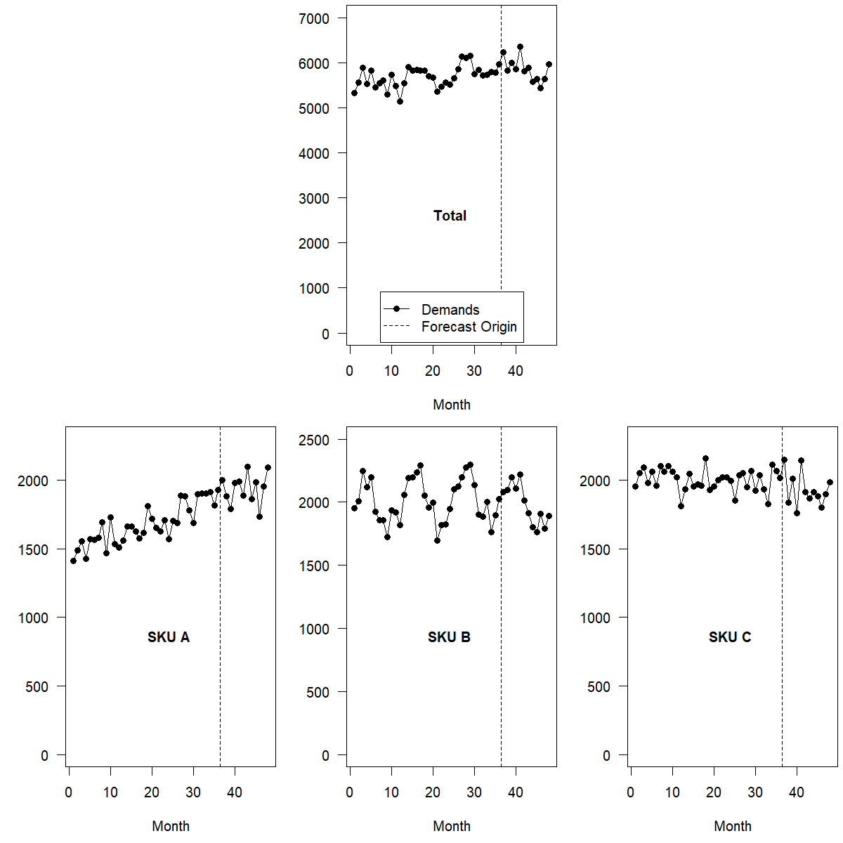
Figure 13.2: An example hierarchy with three SKUs’ time series
Bottom-up forecasting
The simplest form of hierarchical forecasting is the bottom-up approach. This method works just as it sounds: we take the time series at the lowest hierarchical level, forecast each of these series separately, and then aggregate the forecasts up to the desired level of aggregation (without separately forecasting at the higher levels). Many firms use this method without explicitly identifying it as such. The total demand forecast is the sum of product forecasts – a simple bottom-up procedure.
Bottom-up forecasting also works in situations where we do not simply sum up lower level time series but require multiplers, as in bills of material. In the muffin-baking example above, the bakery would forecast its sales of blueberry and chocolate chip muffins separately. It then multiplies each forecasted number with the specific quantity of flour going into each separate muffin and sums the separate forecasts for flour to get a final aggregate flour demand forecast. This is an example of bottom-up forecasting with conversion factors (flour volume per dozen muffins).
One advantage of this approach lies in its simplicity. Implementing this method is effortless, and the bottom-up forecasting process offers little opportunity for mistakes. In addition, it is also straightforward to explain this approach to a non-technical audience. Further, the method is very robust: even if we badly misforecast one series, we limit our error to this series and the levels of aggregation above it – the grand total will not be perturbed a lot. In addition, bottom-up forecasting works very well with causal forecasts since you are more likely to know the value of your causal effect, like the price, on the most fine-grained level. Finally, bottom-up forecasting can lead to fewer errors in judgment for non-substitutable products, increasing the accuracy of forecasts if human judgment plays an essential role in the forecasting process (Kremer et al., 2016).
However, bottom-up forecasting also offers challenges. We lose reliability as we “zoom in” and may miss the forest among the trees. The more granular and disaggregated the historical time series are, the more intermittent they will be, especially if we cross different hierarchies. On a single SKU × store × day level, many demand histories will consist of little else but zeros. On a higher aggregation level, for example, SKU × week, the time series may be more regular. Forecasts for intermittent demands are notoriously tricky, unreliable, and noisy (see Chapter 12). Second, while some causal factors are well defined on a fine-grained level, general dynamics are tough to detect. For instance, a set of time series may be seasonal, but the seasonal signal may be weak and difficult to detect and exploit. Seasonality may be visible on an aggregate level but not at the granular level. In such a case, fitting seasonality on the lower level may even decrease accuracy (Kolassa, 2016b).
Figure 13.3 shows bottom-up forecasting applied to the example hierarchy from Figure 13.2. The trend in SKU A and the seasonality in SKU B are captured well, and the forecast on the Total level consequently shows both a weak trend and weak seasonality. However, the total forecast is too high, since the trend forecast for SKU A overshot its future demand.
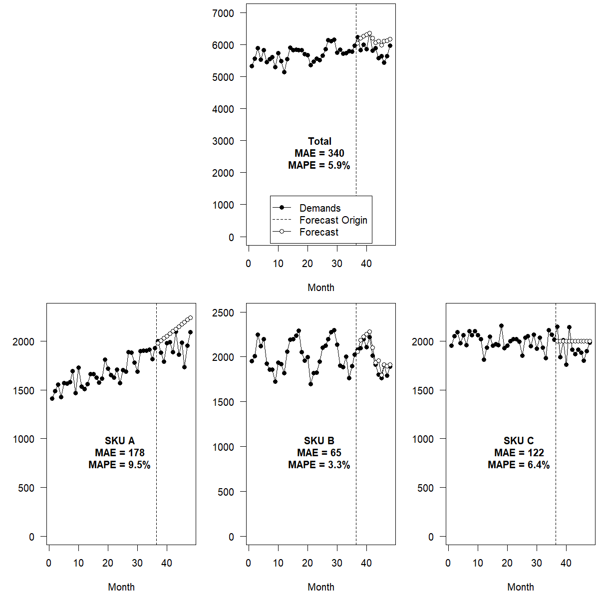
Figure 13.3: Bottom-up forecasts
Top-down forecasting
Top-down is a slightly more complex approach than bottom-up forecasting. As the name implies, this process means that we forecast at the highest level of the hierarchy (or hierarchies), then disaggregate forecasts down to lower levels.
What is more complex about top-down forecasting? We need to decide how to disaggregate the higher-level forecasts. And this, in turn, is nothing more than forecasting the proportions in which, say, different SKUs will make up total category sales in a given month. Of course, these proportions could change over time.
One way of forecasting proportions is to disregard possible changes in proportions over time. Following this approach, we could disaggregate the sum by calculating the proportions of all historical sales. This approach is also called “disaggregation by historical proportions” and assumes that historical proportions will continue to be valid in the future. We could instead use only the most recent proportions to disaggregate our forecasts (“disaggregation by recent proportions”). Doing so would allow us to be more responsive to changes in our data. Such an approach assumes constantly changing proportions. The debate from Section 7.3 on stability vs. change is as valid in this context as before.
Sometimes, these proportions are relatively well-known and stable quantities. For example, the distribution of shoe sizes does not change much over time. Thus, we can readily use these persistent proportions when disaggregating demand for a particular shoe to the shoe \(\times\) size level.
Alternatively, we could forecast the higher level as above but also forecast lower-level demand series and break down total forecasts proportionally to the lower-level forecasts (“disaggregation by forecasted proportions”). Any number of forecast algorithms, seasonal or not, trended or not, could be used for this purpose. We do not need to determine the forecasts for the top level (used to forecast total demands) with the same method as those for lower levels (which we only use to derive proportions).
As you can tell, top-down forecasting can become more complex than bottom-up forecasting and requires careful consideration. On the plus side, top-down forecasting is still relatively simple to use and explain. And in explaining an implementation of the process, the question of how to forecast the disaggregation proportions (a more complex issue) can often be relegated to a technical footnote. Further, top-down forecasting can better incorporate inter-relationships between time series, particularly in the context of substitutable products (Kremer et al., 2016).
On the downside, the other advantages and disadvantages of top-down forecasting mirror those of the bottom-up approach. Whereas bottom-up forecasting is robust to single misforecasts, top-down forecasting faithfully pushes every error on the top level down to every other level.
Furthermore, top-down forecasting often gets the total forecast right at the expense of lower-level errors. How this process breaks the sum into its parts depends on how we forecast future proportions. Suppose demand gradually shifts from SKU A to SKU B because of changes in customer taste. In that case, we need to include this shift explicitly in our proportion estimates, or the disaggregated forecasts will not benefit from this critical information.
While causal factors like prices are well defined for bottom-up forecasting (although their effect may be hard to detect, see Kolassa, 2016b), they are not necessarily as well defined for top-down forecasting. Prices are defined on single SKUs, not on “all products” level. We could use averages of causal factors, for example, average prices in product hierarchies. However, if we use unweighted averages, we relatively overweight slow-selling products. Suppose we use weighted averages of prices, for example, weighting each SKU’s price with its sales to account for its importance in the product hierarchy. In that case, we have to solve the problem of how to calculate these weights for the forecast period. Calculating a weighted average price may be tempting, where we weigh each SKU’s price with its forecasted sales. However, such an approach would be putting the cart before the horse, since forecasting the bottom levels is exactly what we are trying to do.
Figure 13.4 shows top-down forecasting, using disaggregation by historical proportions, applied to the example hierarchy from Figure 13.2. As the trend and seasonal signal are weak at the Total level, the automatic model selection picks Single Exponential Smoothing. Consequently, neither the total forecast nor the disaggregated forecasts on the SKU level exhibit trend or seasonality. Top-down forecasting is inappropriate in this example because the bottom-level time series show obvious but different signals (trend in SKU A, seasonality in SKU B, nothing in SKU C). If the bottom-level series exhibit similar but weak signals, top-down forecasting may perform better than bottom-up (Kolassa, 2016a).
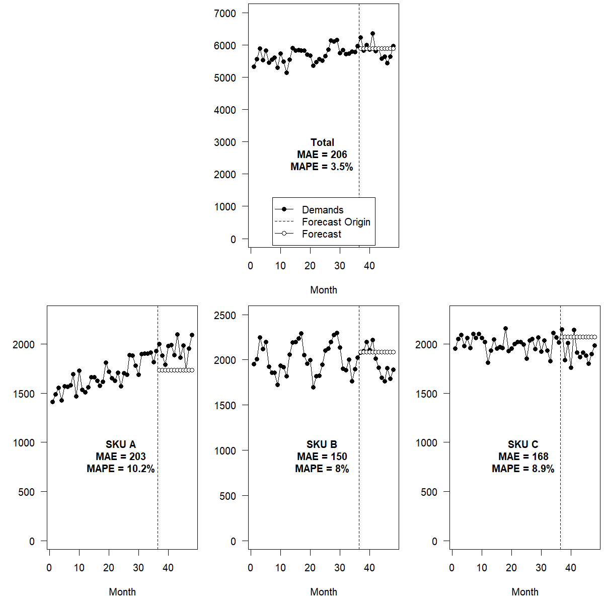
Figure 13.4: Top-down forecasts
Middle-out forecasting
Middle-out forecasting is a middle road between bottom-up and top-down forecasting. Pick a “middle” level in your hierarchy. Aggregate historical data up to this level. Forecast. Disaggregate the forecasts back down, and aggregate them up as required.
This approach combines both the advantages and disadvantages of bottom-up and top-down forecasting. Demands aggregated to a middle level in the hierarchy will be less sparse than on the bottom level, leading, e.g., to better-defined seasonal signals. It may also be easier to derive aggregate causal factors when going to a middle level than when going to the top level. For instance, if all products of a given brand have a “20% off” promotion, we can aggregate historical demands to total brand sales and apply a common “20% off promotion” predictor to the aggregate. (However, as above, we would need to explicitly model differential sensitivity to price reductions for the different SKUs in the brand – a simple approach would yield the same forecasted uplift for all products.)
Once we have the forecasts on a middle level, aggregating them up is just as simple as aggregating bottom-level forecasts in a bottom-up approach. And conversely, disaggregating middle-level forecasts down to a more fine-grained level is similar to disaggregating top-level forecasts in a top-down approach: we again need to decide on how to set disaggregation proportions, for instance, (the most straightforward way) doing disaggregation by historical proportions.
Optimal reconciliation forecasting
One recently developed approach, and an entirely novel way of looking at hierarchical forecasting, is the optimal reconciliation approach (Hyndman et al., 2011; Hyndman and Athanasopoulos, 2014). The critical insight underlying this approach is to return to the consistency problem of hierarchical forecasting. If we separately forecast all our time series on all aggregation levels, then the point forecasts will not be coherent. They will not “fit” together. In that case, we can calculate a “best (possible) fit” between forecasts made directly for a particular hierarchical level and indirectly by either summing up or disaggregating from different levels, using methods similar to regression. We will not go into the statistical details of this method and refer interested readers to Hyndman et al. (2011).
Calculating optimally reconciled hierarchical forecasts provides several advantages. One benefit is that the final forecasts use all component forecasts on all aggregation levels. We can use different forecasting methods on different levels or even mix statistical and judgmental forecasts. Thus, we can model dynamics on the levels where they are best fitted, for example, price influences on a brand level and seasonality on a category level. We, therefore, do not need to worry about making hard decisions about how to aggregate causal factors. If it is unclear how to aggregate a factor, we can leave it out in forecasting on this particular aggregation level. And it turns out that the optimal reconciliation approach frequently yields better forecasts on all aggregation levels, beating bottom-up, top-down, and middle-out in accuracy because it combines so many different sources of information.
Optimal reconciliation, of course, also has drawbacks. One is that the specifics are harder to understand and communicate than the three “classical” approaches. Another disadvantage is that while it works very well with “small” hierarchies, it quickly poses computational and numerical challenges for realistic hierarchies in demand forecasting, which could contain thousands of nodes arranged on multiple levels in multiple crossed hierarchies. For single (non-crossed) hierarchies or for crossed hierarchies that are all of height 2 (“grouped” hierarchies), one can do clever algorithmic tricks (Hyndman et al., 2016). However, the general case of crossed larger hierarchies is still intractable, and optimal reconciliation was not used by many teams in the recent M5 forecasting competition (Makridakis, Spiliotis, and Assimakopoulos, 2022), presumably because of exactly these computational difficulties.
Figure 13.5 shows optimal combination forecasting applied to the example hierarchy from Figure 13.2. As in bottom-up forecasting (Figure 13.3), the method captures the trend in SKU A and the seasonality in SKU B well. The forecast on the aggregate level consequently shows both a weak trend and weak seasonality. Note that errors for optimal combination forecasts are even lower than those for bottom-up forecasts. This is a frequent finding. Optimal reconciliation tends to be more accurate.

Figure 13.5: Optimal reconciliation forecasts
Optimal reconciliation forecasting for hierarchical time series is implemented in the hts package for R (Hyndman et al., 2021).
Other aspects of hierarchical forecasting
A hierarchy used for forecasting should follow the many-to-one rule: many lower levels group into one higher level, but a lower level should not be part of several higher levels. Forecasting hierarchies are sometimes inherited from other organizational planning processes that do not follow this many-to-one rule. As a result, a product can be, for example, sometimes a part of multiple categories. This issue can lead to double counting and inconsistencies when we sum lower levels into higher levels or disaggregate higher levels into lower levels.
If it looks like one hierarchical node might be a child of multiple parent nodes, that may be a symptom of more than one hierarchy being involved: if a car manufacturer customer active in Germany and the UK is member of both the “automotive” and the “Europe” nodes in our single organizational hierarchy, then the best approach is to explicitly create separate (but crossed) customer and geographical hierarchies.
Hierarchical structures allow forecast improvements even if we are not interested in hierarchical forecasts per se. For example, we may only need SKU-level forecasts but still be interested in whether product groups allow us to improve these SKU-level forecasts. For instance, estimating multiplicative seasonality components at a higher level is often helpful if we are confident that all lower levels should exhibit this seasonality. These time series components are much more apparent at that higher level. Once estimated, we can apply them directly to forecast (deseasonalized) lower-level series. In other words, while seasonality is estimated top-down, the remaining forecast (factoring in these seasonal factors) can be done bottom-up. Mohammadipour et al. (2012) explain this approach in more depth. We could use the same method to calculate the effects of trends, promotions, or any other dynamic on an aggregate level, even if we are not interested in aggregate forecasts per se.
One crucial point to remember when forecasting hierarchical data is that structural hierarchies are often not set up with forecasting in mind. For instance, products grouped by suppliers may sort different varieties of apples into different hierarchies, although they appear the same to customers and would profit from hierarchical forecasting as discussed below. One retailer may divide his fruit and produce first into organic vs. conventional and then into the different varieties of fruit, whereas another retailer may first group by fruit and divide organic vs. conventional bananas only at the bottom of the hierarchy. Since the organic and conventional varieties of the same fruit may share similar seasonal patterns, making the organic vs. conventional distinction lower in the hierarchy may help improve forecasts, because then the two varieties of banana are closer together in the hierarchy and can share information. It may thus be worthwhile to create dedicated “forecasting hierarchies” and to check whether these improve forecasts (Mohammadipour et al., 2012).
13.3 Temporal hierarchies and aggregation
Increasing computing power and improvements in database architectures allow us to capture and store data in increasingly finer temporal granularity, such as point-of-sales transaction timestamps in a supermarket and patients’ exact arrival times in a hospital. While point-of-sales systems record sales the second they are made, we require forecasts at coarser time granularities. Generally, the time unit registered will not match the time unit necessary for decision-making and planning. We thus often first have to translate the raw time series of recorded data at higher frequencies (e.g., daily/hourly) into lower frequency forecasts (e.g., weekly/monthly totals).
We then face the challenge that different decisions in the company require forecasts on different temporal granularities. For example, a supply chain manager at a regional warehouse may make weekly decisions for distribution, monthly decisions for stock replenishment, and yearly decisions for purchasing. At a brick and mortar retailer, the store manager needs hourly forecasts for planning production at the deli counter and daily forecasts for replenishing the shelves, whereas the promotion planner looks at weekly total forecasts when planning offers. An online fashion retailer may need forecasts of daily goods movements to schedule the warehouse workforce and will also need forecasts for the entire fashion season, ranging from a few weeks to a few months, to procure products in the countries of origin.
Thus, temporal hierarchies are very similar to the structural hierarchies discussed above, and forecasting in temporal hierarchies can be addressed in similar ways – almost. There are two key differences. One is that while structural hierarchies are only present if we have an entire collection of time series, along with their structural hierarchy, a temporal hierarchy is already implicitly given in a single time series: we can consider forecasts on various time granularities even if we have only one series to forecast. The other main difference between temporal and structural hierarchies is the one between non-overlapping and overlapping temporal aggregation: we can aggregate data in consecutive non-overlapping buckets, e.g., monthly data to quarterly totals (see Figure 13.6), but we can also aggregate it into overlapping totals, say of 3-month periods (see Figure 13.7). It turns out that modeling overlapping temporal aggregates may even improve forecasts if we are not interested in the overlapping buckets as an end result (Boylan and Babai, 2016; Rostami-Tabar et al., 2022).
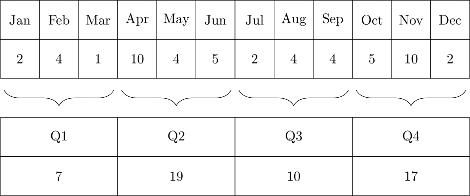
Figure 13.6: Non-overlapping temporal aggregation of monthly demands to quarters
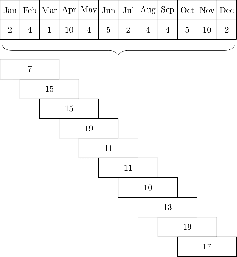
Figure 13.7: Overlapping temporal aggregation of monthly demands to 3-month buckets
Figure 13.8 illustrates a time series of monthly granularity and non-overlapping aggregated series at quarterly and annual levels for retail sales in millions of Australian dollars (Godahewa et al., 2021). Seasonality and trend dominate the monthly and quarterly series. As we increase the granularity to the annual level, the seasonality disappears, while the trend is very apparent.

Figure 13.8: Australia retail sales in millions of Australian dollars. Original time series sampled at a monthly frequency and aggregated at quarterly and annual levels
Applying such a non-overlapping temporal aggregation approach can influence the components of a time series, including seasonality, trend, and autocorrelation. In other words, different aggregation levels can reveal or conceal the various time series components. We generally observe fewer peaks and troughs in low-frequency (aggregated) series than in high-frequency series, i.e., a lower frequency reduces the impact of seasonality. Therefore, while seasonality may be a dominant feature in a higher frequency (e.g., daily) time series, this seasonal pattern can disappear by increasing the aggregation level to a lower frequency (e.g., yearly). The strength of a trend may increase by aggregating the series. We are more likely to see trend patterns in lower-frequency time series. Moreover, autocorrelation patterns can decrease with aggregating series to a lower frequency.
In the case of intermittent demand time series (see Chapter 12), moving from a higher to a lower frequency reduces or even entirely removes the time series intermittency (Nikolopoulos et al., 2011), minimizing the number of periods with zero demands. This form of aggregation can allow the use of conventional forecasting methods in otherwise intermittent series. Figure 13.9 illustrates a time series of spare part sales (Godahewa et al., 2021) at the original monthly and aggregated quarterly and annual levels. We can see how non-overlapping temporal aggregation transforms the time series, leading to fewer zero values for the quarterly and almost no zero values for the annual time series.
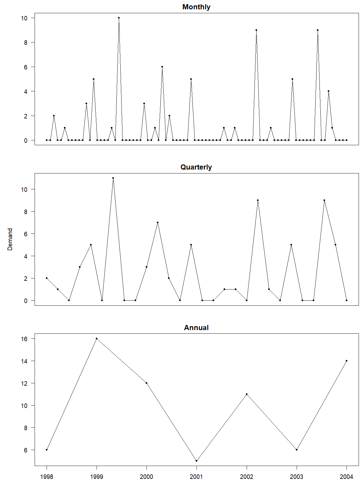
Figure 13.9: A monthly intermittent time series at different levels of non-overlapping temporal aggregation
Forecasts are always necessary at the time unit they are needed for decision-making. But, for example, if we need weekly forecasts and daily data is highly intermittent, a possible approach is to aggregate the daily data into weekly data before forecasting and finally disaggregating the forecast again. Non-overlapping temporal aggregation can thus have its advantages.
We emphasize a few limitations of using a single time unit to generate forecasts:
- The forecast generated at the time unit necessary for decision-making is not necessarily the most accurate one.
- A single time unit ignores time series components at all other levels and does not benefit from such information.
- Two sets of forecasts generated from the same data at different temporal aggregation levels are rarely consistent. For instance, the sum of daily forecasts is likely different from a weekly forecast based on aggregated weekly data. If these two different forecasts inform different decision-making processes, the “weekly” decisions will not be coherent with the “daily” decisions.
Instead of using a single time unit to generate the forecast, we can create multiple time series using non-overlapping temporal aggregation (e.g., monthly, quarterly, yearly), train and create forecasts at each level, and combine available forecasts at multiple levels of aggregation. The key idea is to exploit the information available at various time levels.
The Multi Aggregation Prediction Algorithm (MAPA), introduced by Kourentzes et al. (2014), applies this idea. The MAPA first constructs multiple time series from the original data using non-overlapping temporal aggregation. For example, we sum up our daily demands to create weekly demands. We then forecast each time series separately by fitting an appropriate model (see Chapter 9) to each time series separately. This process would give us daily forecasts (based on daily data) and weekly forecasts (based on weekly data). Next, we would sum up the daily forecasts to create a second weekly forecast, and we disaggregate the original weekly forecast (usually by simply dividing it by the number of workdays) into a second set of daily forecasts. This process would leave us with two weekly forecasts and two sets of daily ones. Last, we would combine the two weekly forecasts and the two sets of daily forecasts by averaging them (or calculating the median) to create one final weekly forecast and one final set of daily forecasts. Figure 13.10 provides an overview of this process.
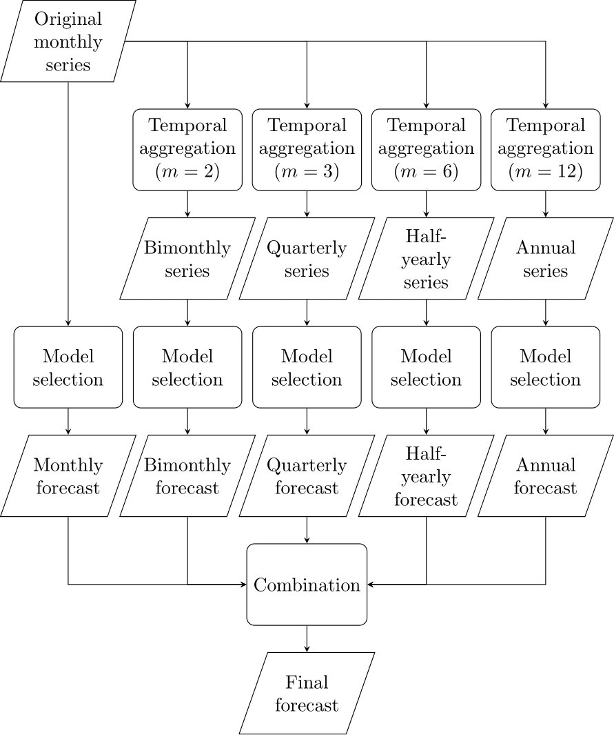
Figure 13.10: The Multi Aggregation Prediction Algorithm (MAPA) applied to a monthly series
A slight complication can arise for seasonal series. Seasonality can quickly disappear for some levels of aggregation. For example, in our daily series, we may have seasonality (demand is always higher on Saturday), which would disappear once we aggregate the data to weekly demand. When applying MAPA and disaggregating the weekly forecast to the daily level, these disaggregated daily forecasts would not exhibit any seasonality. The solution to this problem is to aggregate/disaggregate components, not forecasts. We would think of the disaggregated daily forecasts as level estimates, and average them with the level estimates from directly forecasting at the daily level, then adding the seasonal component at the daily level to derive a combined forecast. MAPA allows us to capture time series components at each temporal aggregation level. The algorithm also benefits from forecast model combination. While MAPA works well with Exponential Smoothing models (so we can combine all the level, trend, and seasonal components), one can also extend the idea to employ other forecasting models – or even apply it to structural instead of temporal hierarchies.
A related approach is the temporal hierarchies process proposed by Athanasopoulos et al. (2017). The idea is to think about the temporal levels as an explicit hierarchy and treat it with the exact same tools as discussed in Section 13.2. Higher frequency time series are at the bottom of this hierarchy (e.g., daily), and lower frequencies (e.g., monthly, quarterly, semi-annual, annual) are at the higher levels. Figure 13.11 shows an example of a temporal hierarchy for a monthly time series with three temporal levels at the monthly, quarterly, and annual levels. For a given forecasting method, we generate forecasts at all levels of the hierarchy and then combine these forecasts to develop reconciled forecasts for all levels.
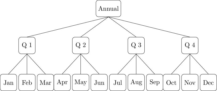
Figure 13.11: An example of a temporal hierarchy for a monthly series with three temporal granularities.
We will not go into the technical details of these approaches – readers can refer to Athanasopoulos et al. (2017) and Kourentzes et al. (2014), or look at the thief (Athanasopoulos et al., 2017; Hyndman and Kourentzes, 2018) and MAPA (Kourentzes and Petropoulos, 2016, 2022; Kourentzes et al., 2014) packages for R.
13.4 When do we not want coherent forecasts?
The chapter so far has been about coherent forecasts, i.e., the situation where the bottom-level forecasts sum up to the single top-level forecast. This requirement is often taken for granted. However, it is not always useful.
The most important example where coherent forecasts do not make sense is in interval or quantile forecasting (see Section 4.2). A 90% quantile forecast for a higher level node in the supply chain is usually much lower than the sum of the 90% quantile forecasts at downstream nodes. Of course, this is as it should be, and it makes perfect sense: noise and variability at the lower level nodes cancel out (sometimes demand is high at node A, but low at node B, or vice versa), so the sum has lower relative variability. As a result, the safety stock required at an upstream node is lower than the sum of safety stocks required at multiple downstream nodes. Thus, it makes no sense to require coherence from prediction intervals or quantile forecasts.
For full predictive densities (see Section 4.3), there is a notion of probabilistic coherence (Panagiotelis et al., 2023). However, this is highly technical and an area of active research.
Finally, there are some subtle points about optimizing hierarchical forecasts with regard to certain error measures. Minimizing the Mean Absolute Percentage Error (MAPE; see Section 17.2) is a target that conflicts with the requirement of coherent forecasts, because the MAPE-optimal forecast is not additive (Kolassa, 2022b). If your bonus is tied to minimizing MAPEs of coherent forecasts, incentives may not be well aligned.
Key takeaways
If you have a small hierarchy and can use dedicated software like R’s
htspackage, or have people sufficiently versed in linear algebra to code the reconciliation themselves, go for the optimal reconciliation approach. If the optimal reconciliation approach is not possible, use one of the other (i.e., bottom-up, top-down or middle-out) methods.You can create time series at multiple temporal levels (daily, weekly, monthly), forecast each series, and reconcile these forecasts using optimal reconciliation.
If you are most interested in the top-level forecasts, with the other levels “nice to have” or are worried about extensive substitutability among your products, use top-down forecasting.
If you are most interested in the bottom-level forecasts, with the other levels “nice to have,” or many of your products are not substitutes, use bottom-up forecasting.
If you can’t decide, use middle-out forecasting. Either pick a middle level that makes sense from a business point of view, for example, the level in the product hierarchy at which you plan marketing activities, or try different levels and look at which one yields the best forecasts overall.
Never be afraid of including hierarchical information, even if you are not interested in higher aggregation-level forecasts. It may improve your lower-level forecasts.
Consider creating additional “forecasting hierarchies” if that helps to do the job.
Do not reconcile hierarchical forecasts blindly. Not all forecasts need to be coherent.