10 ARIMA models
Besides Exponential Smoothing, so-called ARIMA, or Box–Jenkins models, represent another approach for analyzing time series. ARIMA stands for Autoregressive Integrated Moving Average. These models are popular, particularly among econometric forecasters. As we will see later in this chapter, ARIMA models generalize Exponential Smoothing models.
There is a logic explaining the popularity of ARIMA models: If Exponential Smoothing models are a special case of ARIMA models, then ARIMA models should outperform, or at least perform equivalently to, Exponential Smoothing. Unfortunately, though, this logic does not seem to hold in reality. In large forecasting competitions (Makridakis et al., 1993; Makridakis and Hibon, 2000), Exponential Smoothing models regularly beat ARIMA models in out-of-sample comparisons (Wang et al., 2022). Nevertheless, forecasters continue to use ARIMA models, and this chapter will briefly explore the mechanics of ARIMA time series modeling.
10.1 Autoregression
The first component of an ARIMA model is the autoregressive (AR) component. Autoregression or autocorrelation (see Section 6.5) means that we conceptualize current demand as a function of previous demand. This modeling choice conceptualizes demand slightly differently (though mathematically somewhat similar) than Exponential Smoothing. If we see demand as driven by only the most recent demand, we can write the simplest form of an ARIMA model, also called an AR(1) model, as follows:
\[\begin{equation} \mathit{Demand}_t = a_0 + a_1 \times \mathit{Demand}_{t-1} + \mathit{Error}_t \tag{10.1} \end{equation}\]
Equation (10.1) looks like a regression equation (see Chapter 11), with current demand being the dependent variable and previous demand being the independent variable. AR(1) models can be estimated this way – simply as a regression equation between previous and current demand. One can, of course, easily extend this formulation and add more lagged terms to reflect a dependency of the time series that goes deeper into the past. For example, an AR(2) model would look as follows:
\[\begin{equation} \mathit{Demand}_{t} = a_{0} + a_{1} \times \mathit{Demand}_{t-1} + a_{2} \times \mathit{Demand}_{t-2} + \mathit{Error}_{t} \tag{10.2} \end{equation}\]
Estimating this model again follows a regression logic. Generally, an AR(\(p\)) model is a regression model that predicts current demand with the \(p\) most recent past demand observations.
Trends in a time series are usually filtered out before we estimate an AR model by first-differencing the data. Further, dealing with seasonality in this context of AR models is straightforward. For instance, you can deseasonalize your data before analyzing a time series by taking year-over-year differences. You can also include an appropriate demand term in the model equation. Suppose, for example, we examine a time series of monthly data with expected seasonality. We could model this seasonality by allowing the demand from 12 time periods ago to influence current demand. In the case of an AR(1) model with seasonality, we would write this specification as follows:
\[\begin{align} \mathit{Demand}_{t} = a_{0} + a_{1} \times \mathit{Demand}_{t-1} + a_{12} \times \mathit{Demand}_{t-12} + \mathit{Error}_{t} \tag{10.3} \end{align}\]
10.2 Integration
The next component of an ARIMA model is the I, which stands for the order of integration. Integration refers to taking differences of demand data before analysis, i.e., analyzing not the time series itself but analyzing a time series that has been (possibly repeatedly) differenced. For example, an AR(1)I(1) model would look as follows:
\[\begin{equation} \begin{split} & \mathit{Demand}_{t} - \mathit{Demand}_{t-1} \\ = \; & a_{0} + a_{1} \times \left(\mathit{Demand}_{t-1} - \mathit{Demand}_{t-2}\right) + \mathit{Error}_{t} \end{split} \tag{10.4} \end{equation}\]
To make things simple, the Greek letter Delta (\(\Delta\)) is often used to indicate first differences. For example, one can write \[\begin{align} \Delta \mathit{Demand}_{t} = \mathit{Demand}_{t} - \mathit{Demand}_{t-1} \tag{10.5} \end{align}\]
(Other symbols often seen to indicate differencing are the nabla \(\nabla\), or the backshift operator \(B\), or even a \(D\) for “differencing”.)
Substituting Equation (10.5) into Equation (10.4) then leads to the following simplified form:
\[\begin{align} \Delta \mathit{Demand}_{t} = a_{0} + a_{1} \times \Delta \mathit{Demand}_{t-1} + \mathit{Error}_{t} \tag{10.6} \end{align}\]
Taking first differences means that, instead of examining demand directly, one analyzes changes in demand. As discussed in Chapter 5, this technique may make the time series stationary before running a statistical model. (Note, though, that differencing can only remove one particular kind of non-stationarity, namely, trends.) We can also extend the idea of differencing. For example, an AR(1)I(2) model uses second differences by analyzing
\[\begin{align} \Delta^{2} \mathit{Demand}_{t} = \Delta \mathit{Demand}_{t}- \Delta \mathit{Demand}_{t-1} \tag{10.7} \end{align}\]
which is akin to analyzing the changes in the change in demand instead of the demand itself.
To see how a trended time series becomes stationary through integration, consider the following example of a simple time series with a trend:
\[\begin{align} \mathit{Demand}_{t} = a_{0} + a_{1} \times t + \mathit{Error}_{t} \tag{10.8} \end{align}\]
This time series is not stationary since the mean of the series constantly changes by a factor \(a_1\) in each successive period. If, however, we examine the first difference of the time series instead, we observe that in this case:
\[\begin{equation} \begin{split} & \Delta \mathit{Demand}_{t} \\ = \; & \left(a_{0} - a_{0}\right) + \left(a_{1} \times t - a_{1} \times (t-1)\right) + \left(\mathit{Error}_{t} - \mathit{Error}_{t-1}\right) \\ = \; & a_{1} + \mathit{Error}_{t} - \mathit{Error}_{t-1} \end{split} \tag{10.9} \end{equation}\]
The two error terms in Equation (10.9) are simply the difference between two random variables, which is a random variable in itself. In other words, first differencing turned the time series from a non-stationary trended series into a stationary one with a constant mean of \(a_1\). We illustrate this effect in Figure 10.1. The left part of the figure shows a non-stationary time series with a positive trend. The right-hand side of the figure shows the first differences of the same demand observations. These first differences now represent noise around a mean, thus making the series of first differences stationary.
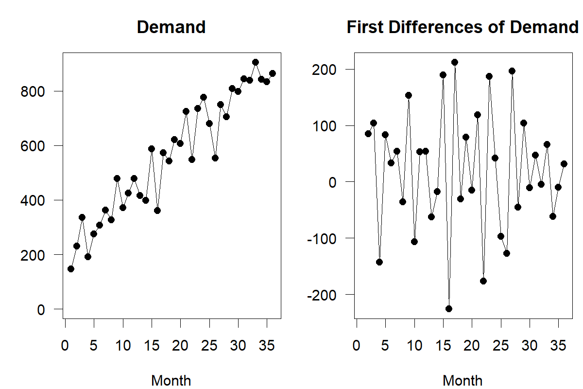
Figure 10.1: First differencing a time series – note the different vertical axes
Sometimes, first-order differencing is insufficient to make a time series stationary, and second- or third-order differencing is needed. Further, some time series require taking the natural logarithm first (which can lead to a more constant variance) or deseasonalizing the series. In practice, forecasters use many manipulations to achieve stationarity of the series, but differencing represents a widespread transformation to achieve this objective.
One can, of course, argue that all these data manipulations distract from the actual objective. In the end, forecasting is about predicting the next demand in a series and not about predicting the next first difference in demand. But notice that we can easily ex-post reverse data manipulations such as first differencing. Suppose you have used an AR(\(p\))I(1) model to predict the next first difference in demand (\(=\mathit{Predicted} \; (\Delta\mathit{Demand})_{t+1}\)). Since you know the currently observed demand, you can construct a forecast for demand in period \(t+1\) by calculating:
\[\begin{align} \mathit{Forecast}_{t+1} = \mathit{Predicted}\; (\Delta\mathit{Demand})_{t+1} + \mathit{Demand}_{t} \tag{10.10} \end{align}\]
10.3 Moving averages
Having discussed the I component of ARIMA models, what remains is to examine the moving averages (MA) component. This MA component in ARIMA models should not be confused with the moving averages forecasting method discussed in Section 9.1! This component represents an alternative conceptualization of serial dependence in a time series – but this time, the subsequent demand does not depend on the previous demand but on the previous error, that is, the difference between what the model would have predicted and what we have observed. We can represent an MA(1) model as follows:
\[\begin{align} \mathit{Demand}_{t} = a_{0} + a_{1} \times \mathit{Error}_{t-1} + \mathit{Error}_{t} \tag{10.11} \end{align}\]
In other words, instead of seeing current demand as a function of previous demand, we conceptualize demand as a function of previous forecast errors. The difference between autoregression and moving averages, as we shall see later in this chapter, essentially boils down to a difference in how persistent random shocks are to the series. Unexpected shocks tend to linger long in AR models but more quickly disappear in MA models. MA models, however, are more difficult to estimate than AR models. We estimate an AR model like any standard regression model. However, MA models have a chicken-or-egg problem: one has to create an initial error term to estimate the model, and all future error terms will directly depend on what that initial error term is. For that reason, MA models require estimation with more complex maximum likelihood procedures instead of the regular regression we can use for AR models.
MA models extend similarly to AR models do. An MA(2) model would see current demand as a function of the past two model errors, and an MA(\(q\)) model sees demand as a function of the past \(q\) model errors.
More generally, when combining these components, one can see an ARIMA(\(p, d, q\)) model as a model that looks at demand that has been differenced \(d\) times, where this \(d\)th demand difference is seen as a function of the previous \(p\) (\(d\)th) demand differences and \(q\) forecast errors. Quite obviously, this is a very general model for demand forecasting, and selecting the right model among this infinite set of possible models becomes a key challenge. One could apply a “brute force” technique, as in Exponential Smoothing, and examine which model among a wide range of choices fits best in an estimation sample. Yet, unlike in Exponential Smoothing, where the number of possible models is limited, there is a nearly unlimited number of models available here since one could always go further into the past to extend the model (i.e., increase the orders \(p\), \(d\) and \(q\)).
10.4 Autocorrelation and partial autocorrelation
Important tools forecasters use to analyze a time series, especially in ARIMA modeling, are the autocorrelation function (ACF) and the partial autocorrelation function (PACF), as well as information criteria, which we consider in Section 10.5.
For the ACF, one calculates the sample correlation (e.g., using the =CORREL function in Microsoft Excel) between the current demand and the previous demand, between the current demand and the demand before the previous demand, and so on. Going up to \(n\) time periods into the past leads to \(n\) correlation coefficients between current demand and the demand lagged by up to \(n\) time periods (see Section 6.5). Autocorrelations are usually plotted against lag order in a barplot, the so-called autocorrelation plot. Figure 10.2 contains an example of such a plot. An added feature in an autocorrelation plot is a horizontal bar, which differentiates autocorrelations that are statistically significant from non-significant ones, that is, autocorrelation estimates that are higher (or lower, in the case of negative autocorrelations) than we would expect by chance. This significance test can sometimes help identify an ARIMA model’s orders \(p\) and \(q\).
The PACF works similarly. We estimate first an AR(1) model, then an AR(2) model, and so on, and always record the regression coefficients of the last term we add to the equation. These partial autocorrelations are again plotted against the lags in a barplot, yielding the partial autocorrelation plot.
To illustrate how to calculate the ACF and the PACF, consider the following example. Suppose we have a demand time series and calculate the correlation coefficient between demand in a current period and the period before (obtaining \(r_1 = 0.84\)), as well as the correlation coefficient between demand in a current period and demand in the period before the previous one (obtaining \(r_2 = 0.76\)). The first two entries of the ACF are then 0.84 and 0.76. Suppose now that we additionally estimate two regression equations:
\[\begin{equation} \mathit{Demand}_{t} = \mathit{Constant}_1 + \theta_{1,1} \times \mathit{Demand}_{t-1} + \mathit{Error}_{1,t} \end{equation}\] and \[\begin{equation} \begin{split} & \mathit{Demand}_{t} \\ = \; & \mathit{Constant}_2 + \theta_{2,1} \times \mathit{Demand}_{t-1} + \theta_{2,2} \times \mathit{Demand}_{t-2} + \mathit{Error}_{2,t}. \end{split} \end{equation}\]
Suppose that the results from this estimation show that \(\theta_{1,1} = 0.87\) and \(\theta_{2,2} = 0.22\). The first two entries of the PACF are then 0.87 and 0.22.
We can use the ACF to differentiate MA(1) and AR(1) processes from each other and differentiate both of these processes from demand, representing simple draws from a distribution without any serial dependence. To illustrate this selection process, Figure 10.2 contains the time series and ACF plots of a series following an AR(1) process, an MA(1) process, and data that represents simple draws from a normal distribution. We generated all three series using the same random draws to enhance comparability. You can see that the MA(1) series and the normal series look very similar. Only a comparison of their ACFs reveals that while the normally distributed demand shows no autocorrelation in any time lag, the MA(1) series shows an autocorrelation going back one time period (but not further). The AR(1) process, however, looks very distinct. Shocks from the series tend to throw the series off from the long-run average for more extended periods. In other words, if demand drops, it will likely stay below average for some time before it recovers. This distinctive pattern is visible in the ACF for the AR(1) process; the autocorrelation coefficients in the series are present in all four time lags depicted, though they slowly decrease as the time lag increases.
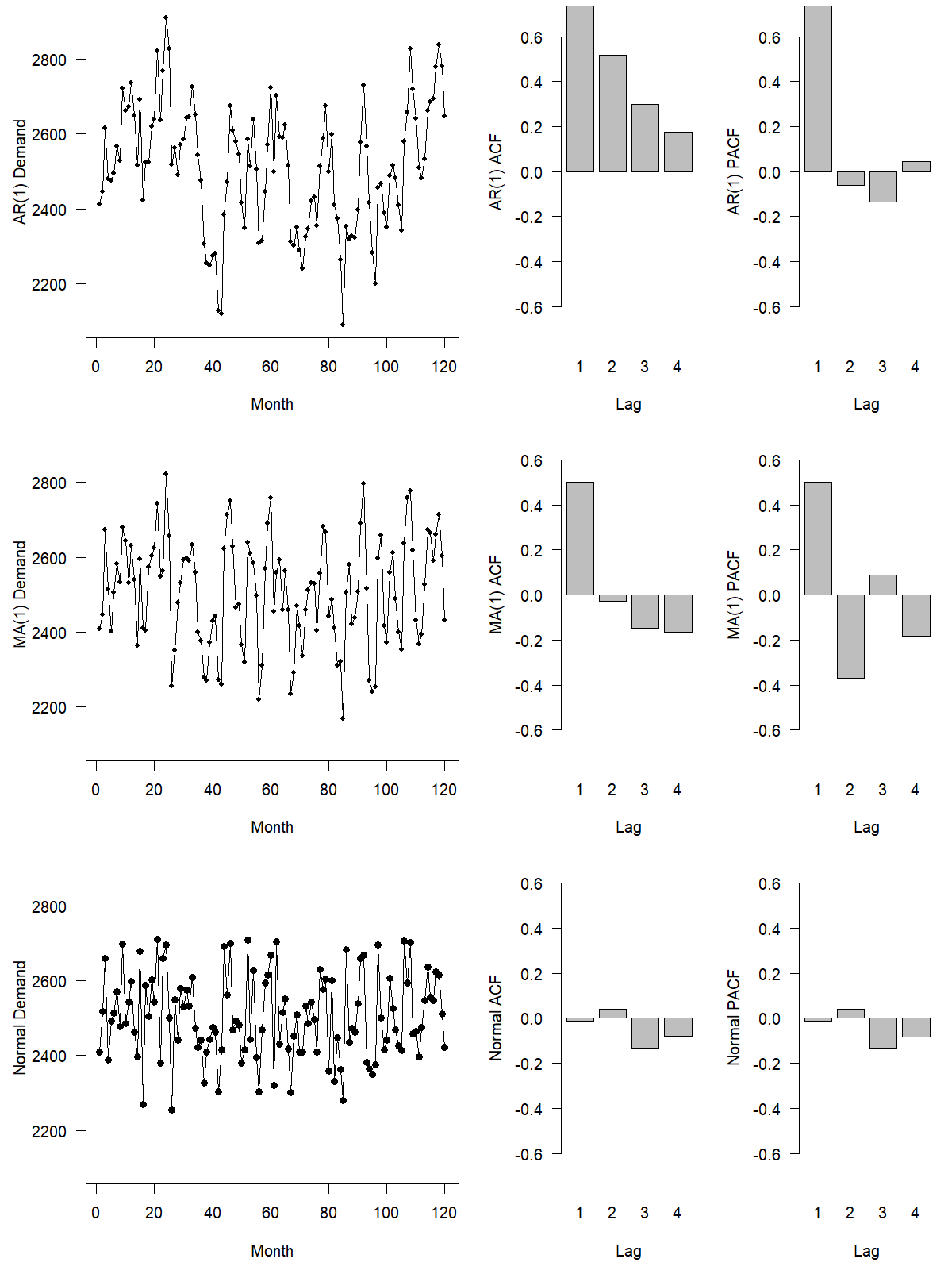
Figure 10.2: Autoregressive (AR), Moving Average (MA) and white noise series with their ACF and PACF
10.5 Information criteria
As discussed above, we can use (P)ACF plots to identify the orders of pure AR(\(p\)) and pure MA(\(q\)) processes and to distinguish these from each other. However, (P)ACF plots are not helpful for identifying general ARIMA(\(p,d,q\)) processes with both \(p,q>0\) or \(d>0\). Since, in practice, we never know beforehand whether we are dealing with a pure AR(\(p\)) or MA(\(q\)) process, the use of (P)ACF plots in order selection is limited (Kolassa, 2022c). For order selection in this more general case, one uses information criteria.
Information criteria typically assign a quality measurement to an ARIMA model fitted to a time series. This value has two components. One is how well the model fits the past time series. However, since we can always improve model fit by simply using a more complex model (which will lead quickly to overfitting and bad forecasts, see Section 11.7), information criteria also include a penalty term that reduces the value for more complex models. Different information criteria differ mainly in how exactly this penalty term is calculated.
The most used information criteria are Akaike’s information criterion (AIC) and the Bayes information criterion (BIC). These two information criteria (and other more rarely used ones) have different statistical advantages and disadvantages, and neither one is “usually” better in choosing the best forecasting model.
Finally, neither the (P)ACF nor information criteria are of any use in selecting the order of integration, i.e., the middle \(d\) entry in an ARIMA(\(p,d,q\)) model. For this, automatic ARIMA model selection typically uses unit root tests.
10.6 Discussion
One can show that using single Exponential Smoothing as a forecasting method is essentially equivalent to using an ARIMA(\(0,1,1\)) model as a forecasting method. With optimal parameters, the two series of forecasts produced will be the same. The apparently logical conclusion is that since ARIMA(\(0,1,1\)) models are a special case of ARIMA(\(p, d, q\)) models, ARIMA models represent a generalization of Exponential Smoothing and thus must be more effective at forecasting.
While this logic is compelling, it has not withstood empirical tests. Large forecasting competitions have repeatedly demonstrated that Exponential Smoothing models tend to dominate ARIMA models in out-of-sample comparisons (Makridakis and Hibon, 2000; Makridakis, Spiliotis, and Assimakopoulos, 2022), although ARIMA has performed well in quantile forecasting in the M5 competition (Makridakis, Petropoulos, et al., 2022). It seems that Exponential Smoothing is more robust. Further, with the more general state space modeling framework (Hyndman et al., 2008), the variety of Exponential Smoothing models has been extended such that many of these models are not simply special cases of ARIMA modeling anymore. Thus, ARIMA modeling is not necessarily preferred as a forecasting method in general; nevertheless, these models continue to enjoy some popularity.
ARIMA modeling is a recommended forecasting approach for a series showing short-term correlation and not dominated by trend and seasonality. However, forecasters using the method require technical expertise to understand how to carry out the method (Chatfield, 2007).
In using ARIMA models, one usually does not need to consider a high differencing order. We can model most series with no more than two differences (i.e., \(d \le 2\)) and AR/MA terms up to order five (i.e., \(p, q \le 5\)) (Ali et al., 2012).
ARIMA models focus on point forecasts, although they can also output prediction intervals and predictive densities based on an assumption of constant-variance Gaussian errors. A similar class of models, called Generalized Autoregressive Conditional Heteroscedasticity (GARCH) models, focuses on modeling the uncertainty inherent in forecasts as a function of previous shocks (i.e., forecast errors). Forecasters use these models in stock market applications. They stem from the observation that large shocks to the market create more volatility in the succeeding periods. The key to these models is to view the variance of forecast errors not as fixed but as a function of previous errors, effectively creating a relationship between previous shocks to the time series and future uncertainty of forecasts. GARCH can be combined with ARIMA models since the former technique is focused on modeling a distribution’s variance while the latter models the mean. An excellent introduction to GARCH modeling is given in Engle (2001) and Batchelor (2010).
ARIMA models, with automatic order selection (“auto-ARIMA”) are implemented in the forecast (Hyndman et al., 2023) and the fable (O’Hara-Wild et al., 2020) packages for R. The pmdarima package for Python (T. G. Smith et al., 2022) ports this functionality from the R packages.
Key takeaways
ARIMA models explain time series based on autocorrelation, integration, and MAs. We can apply them to time series with seasonality and trend.
These models have not performed exceptionally well in demand forecasting competitions but are included in most software packages.
Your software should automatically identify the best differencing, AR, and MA orders based on unit root tests and information criteria and estimate the actual AR and MA coefficients.
ACF and PACF plots are often used in ARIMA modeling to investigate a time series. However, identifying the best ARIMA model based on these plots rarely works.
You will typically not need high AR, MA, or differencing orders for the model to work.