14 Artificial intelligence and machine learning
In this chapter, we will consider “modern” forecasting methods that became more prominent with the advent of Data Science. Umbrella terms used for these methods are “Artificial Intelligence” (AI) and “Machine Learning” (ML). There is no commonly accepted definition of these terms, and boundaries are ambiguous. ARIMA and Exponential Smoothing could certainly be classified as ML algorithms.
A standard categorization in ML distinguishes between supervised and unsupervised learning. The difference between these two approaches lies in whether training data are labeled or not. While supervised learning examines the relationship among labeled data, unsupervised learning examines patterns among unlabeled data. All forecasting methods represent supervised learning, since we train models to known targets (past observed demands) rather than learning without a known target outcome.
14.1 Neural networks and deep learning
Neural Networks (NNs) are Machine Learning algorithms based on simple models of neural processes. Our brains consist of billions of nerve cells, or neurons, which are highly interconnected. When our brain is presented with a stimulus, e.g., an image or scent of a delicious apple, neurons are “activated.” These activated neurons in turn activate other connected neurons through an electrical charge. Over many such stimuli, patterns of connections emerge and change.
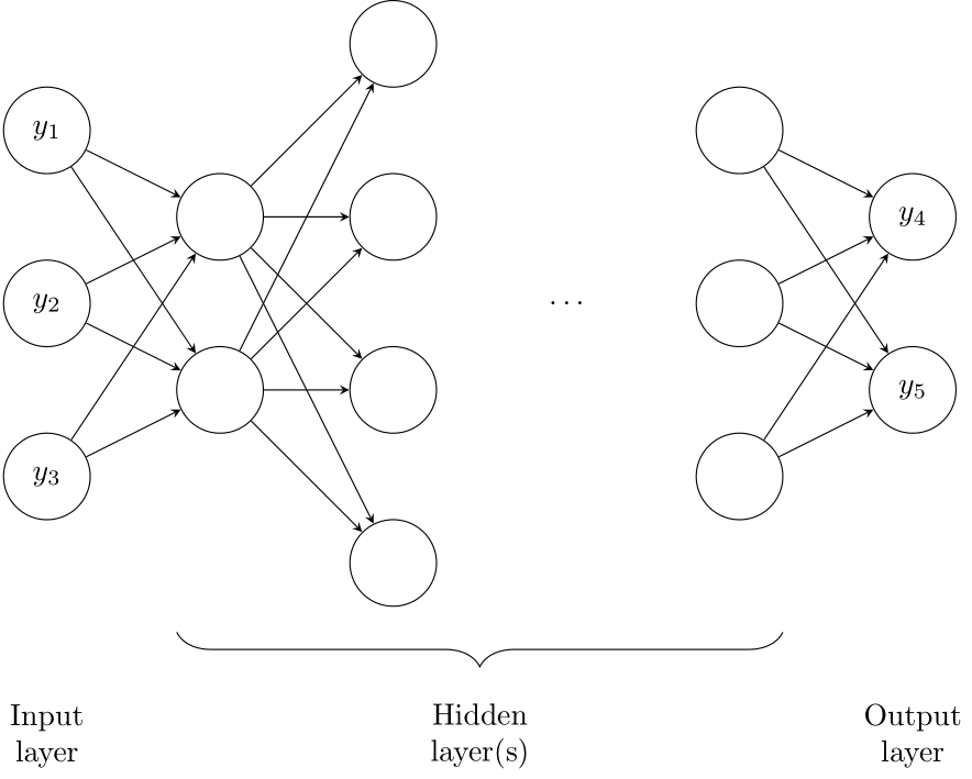
Figure 14.1: A neural network
NNs (the computer kind, see Figure 14.1) imitate this process. They are initialized with an architecture specifying how abstract “neurons” are arranged and interconnected. Typically, neurons are set up in layers, with neurons in neighboring layers connected. An input layer of neurons gets fed input data. This input layer is connected to one or multiple hidden layers. The last hidden layer is connected to an output layer. The number of such layers is called the depth of the network. The term Deep Learning refers to NNs with many layers, in contrast to simpler architectures with only a few layers.
To train such an NN, we present it with inputs, e.g., the historical observations of a time series, and an output, e.g., the subsequent values of the series. The training algorithm adjusts the strengths of the connections between the neurons to strengthen the association between the inputs and the output. This step is repeated with many input-output pairs in the training data. Once the network has “learned” the association between an input and the corresponding output, we can present it with a new input, e.g., the current value of a time series, and obtain the output the NN associates with that input, e.g., our forecast for a future value of the series. The input to a NN used for forecasting can contain more data than just the historical time series, such as time-constant or time-varying predictor information.
NNs have existed since the 1950s. After some initial enthusiasm, interest waned in these methods as they did not seem to provide practical applications (a period sometimes called an “AI winter”). In recent decades, a combination of theoretical advances in NN training algorithms, more powerful and specialized hardware, and abundant data have fomented an explosion of NN research and applications. NNs are often used in pattern recognition tasks, from image recognition to sound and speech analysis. They can also generate patterns, including Deep Fakes of convincing videos, poems, and solutions to academic exam questions. NNs are also increasingly applied to forecasting tasks.
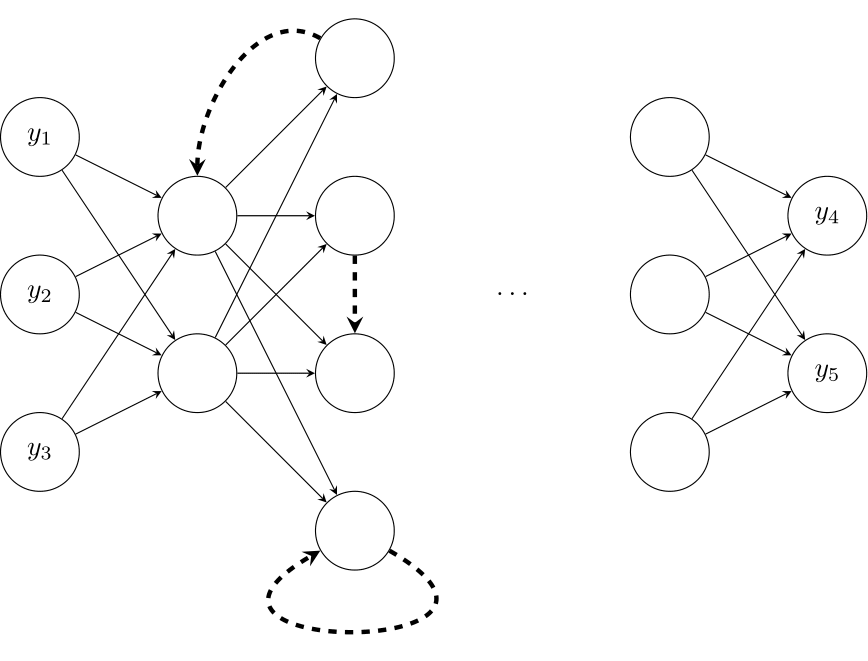
Figure 14.2: A recurrent neural network, with recurrent connections highlighted
The art of using NNs for any task lies in setting up the architecture and in pre-processing the data. For instance, it is often helpful in forecasting to connect “later” layers in the NN to “earlier” layers, which results in a Recurrent Neural Network (RNN, see Figure 14.2). Such a network can be interpreted as representing “hidden states,” i.e., unobserved “states of the world.” More sophisticated versions of RNNs can forget information over time. Such an architecture is known as a Long Short-Term Memory (LSTM) network. Variants of LSTM are the most common NN architecture used in forecasting.
14.2 Tree-based methods and random forests
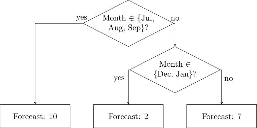
Figure 14.3: A simple decision tree to forecast monthly data
Tree-based methods for forecasting (Januschowski et al., 2022; Spiliotis, 2022) represent a collection of decision rules. An example of such a decision rule is “if the month is July to September, then forecast 10, else forecast 5”. Such decision rules can be applied sequentially. For example, we could refine our decision rule by asking if the month is not July to September, whether it is December or January, and if so, we could forecast 2, and if not, forecast 7. We can increasingly refine our decision rules to yield arbitrarily complex decision chains. If we visualize such a set of decision rules, as in Figure 14.3, it looks like an inverted tree, with the root at the top and branching points below. Each decision point yields such a branching.
Such trees – the specific name for these is Classification And Regression Trees (CARTs) – are trained, or “grown,” by using input and output data. The data are recursively partitioned to minimize the error we would obtain if we used the tree to predict the training data. CARTs overfit easily, i.e., they are prone to follow the noise in the data accidentally. To counteract this, one often limits the maximum depth of the tree or grows it first and then prunes it back by cutting off the bottom branches. Alternatively, one can deal with the overfitting issue by using a Random Forest, see below.
Decision trees can process any predictor. In the example above, we used only the month as a predictor. As a result, we modeled monthly seasonality. We could also include the day of the week for daily data, lagged values of the time series itself, or any other kind of predictor – all we need is that the predictor value is known and available for forecasting.
Random Forests (RFs) are a generalization of CARTs. As the name implies, a RF contains hundreds of trees. In addition, some random mutation is involved in growing a RF by picking a random set out of our training data and growing each tree only on a small random subset of the predictors. This strange double randomization is surprisingly effective at creating a diversity of trees. The forecast from an RF is the average of the forecasts from the component trees. The idea of combining multiple forecasts (here: from the component trees) is an example of ensemble forecasting (see Section 8.6).
14.3 Boosting and variants
We already saw examples of the powerful concept of combining multiple different forecasts via averaging when we encountered Random Forests and Section 8.6. The technique of Boosting represents another way of combining various forecasting methods. Specifically, we first model our time series using any method of choice. We then consider the differences between the original time series and the fitted values, i.e., the model errors. In turn, we predict these errors using another method, typically a very simple one (a so-called weak learner). Then, we iterate this process. The end model and forecast is the sum of the iterative boosted components. Boosting describes how we use and stack specific models in each step. The idea of Boosting (Schapire, 1990) has been around for decades, and several variants have been considered:
Gradient Boosting was proposed by Friedman (2001); here, we replace the differences between the observations and the current fit (the “residuals”) with “pseudo-residuals” involving the derivative of the loss function, which makes the subsequent fitting of weak learners easier.
Stochastic Gradient Boosting (Friedman, 2002) works similarly to Gradient Boosting but only relies on a random sub-sample of the training data in each iteration. This injection of randomness serves a similar purpose as in Random Forests.
(Stochastic) Tree Boosting is a specific kind of (Stochastic) Boosting, where the weak learners fit in each step are simple decision trees, which we have encountered above. The most straightforward possible tree consists of a single split, which is inevitably called a stump.
LightGBM (“Light Gradient Boosting Machine”) and XGBoost (“eXtreme Gradient Boosting”) are specific implementations of Stochastic Tree Boosting, with particular emphasis on efficiency and scalability through distributed learning. These modern methods are frequent top contenders at Kaggle forecasting competitions and dominated the top ranks of the recent M5 time series forecasting competition (Makridakis, Petropoulos, et al., 2022).
14.4 Point, interval and density AI/ML forecasts
While AI/ML methods are often developed to create point forecasts, these methods can also be used to yield interval and density forecasts. For instance, we can train these models to output quantile forecasts using an appropriate pinball loss function (so-called because it resembles the trajectory of a pinball hitting a wall). Thus, one could train an entire group of NNs, and CARTs, each for a different quantile, and get multiple quantile forecasts and the corresponding prediction intervals. Alternatively, we can use AI/ML methods to forecast the parameters of a probability distribution, which gives us total predictive density. One such setup is DeepAR, which uses a NN to predict the parameters of a discrete probability distribution (Salinas et al., 2020).
14.5 AI and ML versus conventional approaches
A critical difference between AI/ML and conventional forecasting methods, such as ARIMA or Exponential Smoothing, is that the conventional methods are linear. AI/ML models are non-linear. For example, if you take a time series, double each value in the series, model it using conventional methods, and create a forecast, your forecast will also be twice as high as the forecasts you would get from the original series. The conventional methods impose a linear structure on the models they generate. AI/ML methods, in contrast, are more flexible. They can model non-linearities.
Allowing for non-linearities sounds like a valuable feature of AI/ML. However, this flexibility comes at a price. AI/ML methods are prone to overfitting, i.e., they tend to follow the noise instead of detecting the signal in the data. Thus, they are more sensitive to random fluctuations in the data. As a result, AI/ML models can produce forecasts that are also highly variable and, therefore, potentially wildly inaccurate. See Section 11.7 on model complexity, overfitting and the bias-variance tradeoff. To counteract this problem, AI/ML methods are typically fed large amounts of data.
AI/ML methods are very data and resource hungry. They require a lot more data input than traditional forecasting methods. They also need much more processing time to train the model before their forecasts make sense. This can lead to an excessive need for computation hours compared to traditional models, leading to cloud computing costs and energy consumption. According to one estimate, moving a large-scale retail forecasting operation from conventional forecasting methods to AI/ML results in extra CO2 emissions due to increased energy use in computation that is equivalent to the annual CO2 production of 89,000 cars (Petropoulos, Grushka-Cockayne, et al., 2022).
If you have a single time series of several years of monthly data, you can easily fit an ARIMA or Exponential Smoothing model to this series and get valuable forecasts. A NN trained on the same series may give highly variable and inaccurate predictions. Thus, AI/ML methods are typically not fitted to a single time series but are instead fitted to a whole set of series. They are global methods, in contrast to traditional methods, which are local to single time series (Januschowski et al., 2020).
This distinction between global and local methods has two consequences. First, local methods can be easily parallelized for higher performance. Global methods need a lot more work to train efficiently. Second, whereas local methods can be understood in isolation (you can look at and understand an ARIMA forecast from a single series), global methods are tough to understand because the forecast for a given series does not only depend on this series itself but also on all the other series that went into training the NN. Recently, academic and practical work has emphasized the importance of “explainable AI” (XAI). This term emphasizes that AI/ML models should be designed in a way as to help humans understand their outputs and predictions. Relatedly, if we want to “debug” a forecast, it is easier to tweak a local method than a global one. If you modify a global method to work better on a particular series, it may suddenly work worse on a seemingly unrelated other series. Usually, many AI/ML models with similar accuracy exist, and one can use the simplest and easiest to interpret and debug among them – a concept known as Rashomon Set Theory (Fisher et al., 2019).
In summary, AI/ML has the potential to achieve better forecasting accuracy than more traditional methods through its greater flexibility, but whether this advantage is realized depends on the time series. For instance, in the M5 forecasting competition, AI/ML had a much greater edge on aggregated data than on the more granular SKU \(\times\) store \(\times\) day level (Makridakis, Petropoulos, et al., 2022). In addition, while AI/ML methods won the M5 competition, conventional methods were competitive: the simplest benchmark, Exponential Smoothing on the bottom level with trivial bottom-up aggregation to higher hierarchy levels, performed better than 92.5% of submissions (Kolassa, 2022a). And the accuracy advantage of AI/ML methods comes at the price of higher complexity, i.e., higher costs. It is not apparent that a more costly, more complex, and more accurate method automatically translates into better business outcomes (Kolassa, 2022a). Thus, although AI/ML has been at the center of every forecaster’s attention, it will likely not be a silver bullet that will solve all our forecasting problems (Kolassa, 2020).
One thing to keep in mind is that computer scientists have primarily driven the development of AI/ML. This poses a problem insofar as forecasting has traditionally been a domain of statisticians and econometricians. One consequence is that AI/ML experts are often unaware of the pitfalls inherent in forecasting in contrast to “traditional” AI/ML use cases, from benchmarking against simple methods to evaluation strategies and adequate evaluation datasets (Hewamalage et al., 2022).
In closing, there is one “human factor” difference between the two approaches to forecasting: the traditional methods are more statistical. They are less in vogue than AI/ML. More people are excited about DL and Boosting than about ARIMA and Exponential Smoothing. AI/ML methods are thus far easier to sell to decision-makers, and it may be easier to find people trained in the newer methods than in the conventional ones. Data Scientists trained in AI/ML tend to require a higher salary than statisticians, econometricians, and business analysts trained in the more conventional methods.
Key takeaways
In recent years, Artificial Intelligence (AI) and Machine Learning (ML) methods have captured our attention in forecasting. Examples include Neural Networks, Deep Learning, tree-based methods, Random Forests, and various flavors of Boosting.
AI/ML methods have outperformed “classical” approaches in terms of accuracy for aggregate time series, but performance comparisons at disaggregate and lower levels of time series are much less apparent.
AI/ML methods are non-linear and more complex. They are thus more demanding in terms of data, computing resources, and expertise and need help understanding and debugging.
Whether the improved business outcome through improved accuracy is worth the added complexity and higher Total Cost of Ownership of AI/ML methods merits careful analysis.